
Conditional formatting in Excel is one of the most powerful tools for making your spreadsheets more insightful and easier to read. Instead of manually scanning rows of numbers or text, conditional formatting automatically highlights the most important parts of your data based on rules that you set. With just a few clicks, you can spot trends, identify outliers, or flag potential issues—all without adding a single formula to your worksheet.
For example, imagine managing a budget where any expense over $1,000 turns red, or tracking project deadlines where tasks due this week are highlighted in yellow. Conditional formatting allows you to create these kinds of dynamic visual cues, making your data tell a story at a glance. Whether you’re a beginner just learning Excel or an advanced user building dashboards, mastering conditional formatting can transform how you work with spreadsheets.
What is Conditional Formatting in Excel?
Conditional formatting in Excel is a feature that applies formatting (such as colors, icons, or data bars) to cells based on specific conditions or rules. This helps in:
- Highlighting key data points (e.g., highest or lowest values).
- Finding and formatting errors or anomalies in datasets.
- Making reports and dashboards visually appealing and easy to interpret.
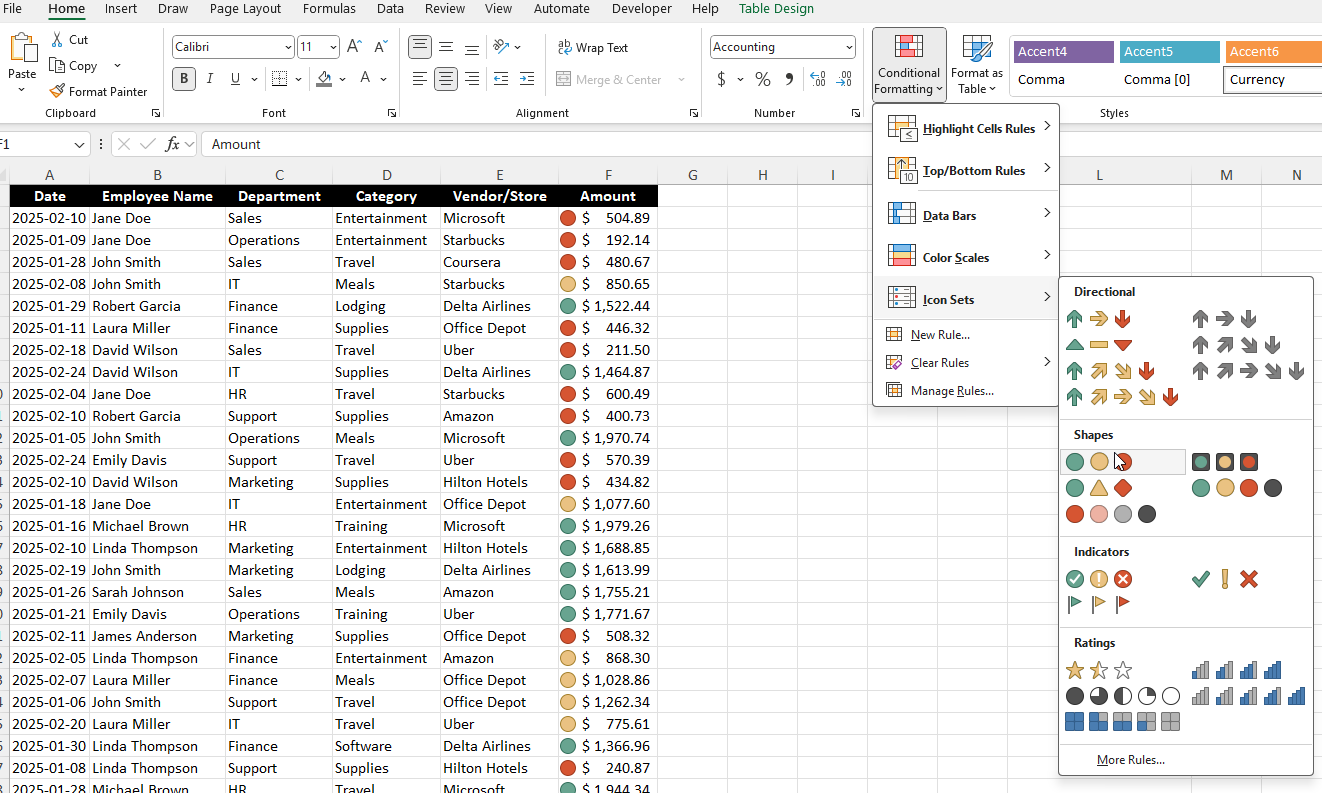
To access conditional formatting, navigate to Home > Conditional Formatting on the Excel ribbon.
General Conditional Formatting Rules in Excel
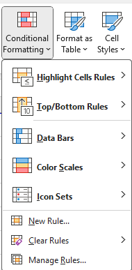
Excel provides several built-in conditional formatting rules, which can be applied with just a few clicks:
Highlight Cells Rules
These rules apply formatting to cells based on their values.
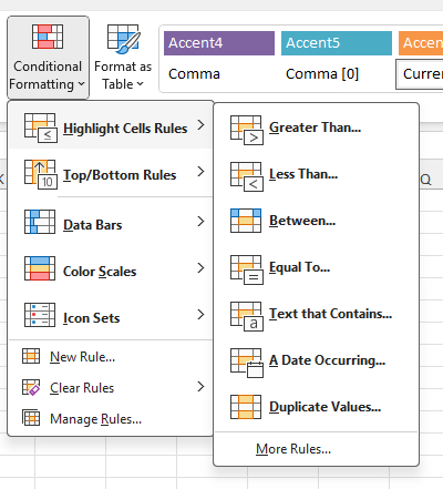
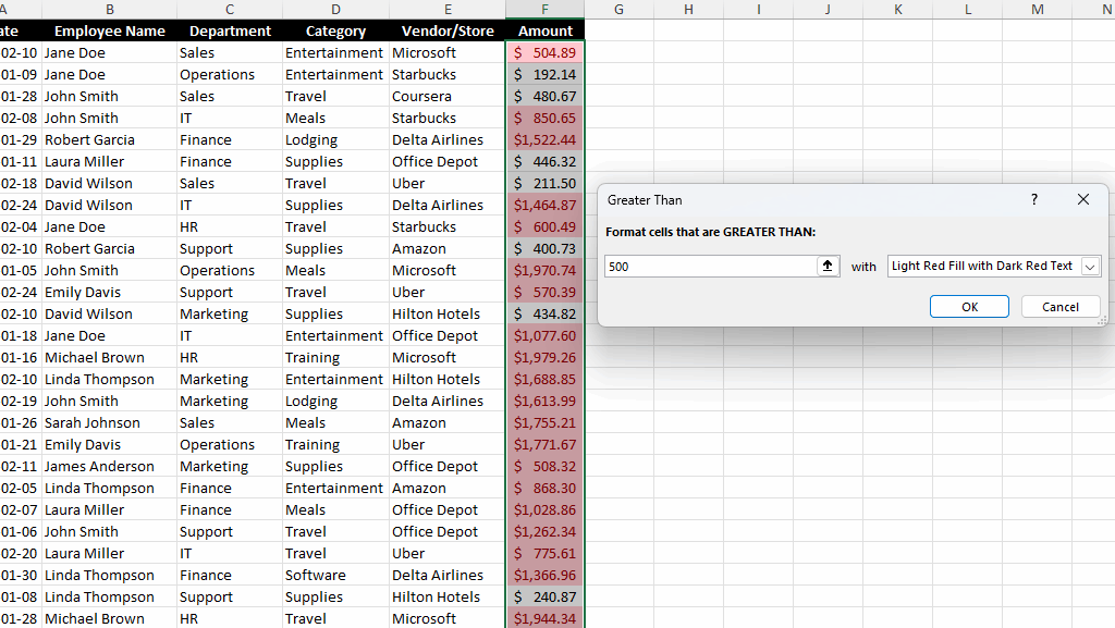
- Greater Than / Less Than: Highlights numbers above or below a certain threshold. In the below data set, all the values that are greater than $500 are highlighted.
- Equal To: Highlights cells that contain a specific value. In the example below, when the Vendor is equal to Office Depot, the cell is highlighted in yellow.

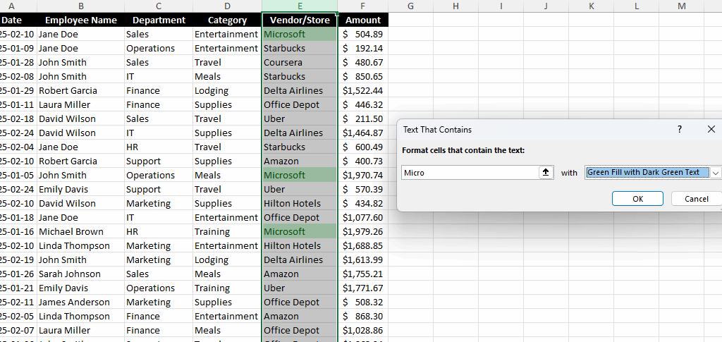
- Text That Contains: Applies formatting to cells that contain certain text. This is useful if you are looking for partial matches. In the below example, any Vendor which contains the word ‘Micro’ is highlighted in green.
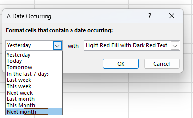
- Dates Occurring: This is useful for highlighting recent, upcoming, or past dates. And the values are dynamic and will change based on the current date.
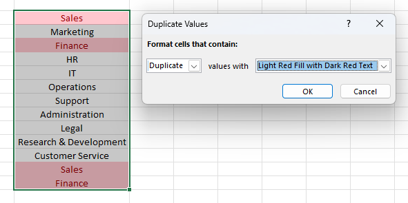
- Duplicate Values: Conditional formatting can help with quickly identifying values in a range of data, showing when there are duplicates found. Below, I’ve highlighted any duplicate values in red.
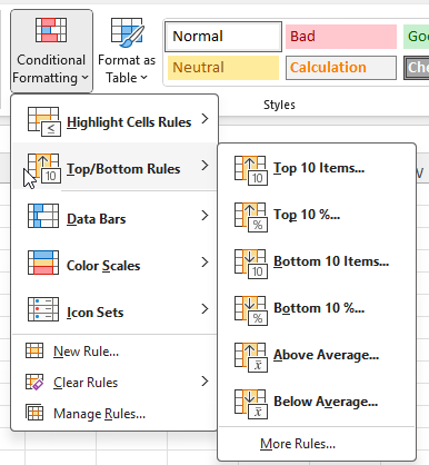
Top/Bottom Rules
In addition to just highlighting specific values, duplicates, or ranges of dates, you can also use conditional formatting to analyze data for you. Here are some of the pre-set options you can highlight:
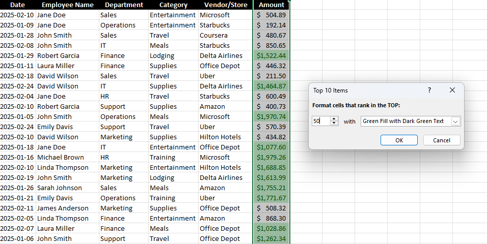
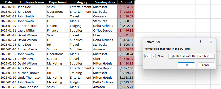
- Top 10 Items / Bottom 10 Items: This option highlights the highest or lowest values in a dataset. While it says the top or bottom 10, this can be modified to show a different number. Below, I’ve highlighted the top 50 largest values in green.
- Top 10% / Bottom 10%: This highlights values that fall in the top or bottom 10%. While the default is to look at the top or bottom 10%, you can change this percentage to whatever cutoff point you want. In the below screenshot, I’ve set the cutoff to 25, to highlight the bottom 25% of values in the data set. By doing this, it’s easy to highlight the largest values without first having to calculate what that cutoff point is — Excel does it all.
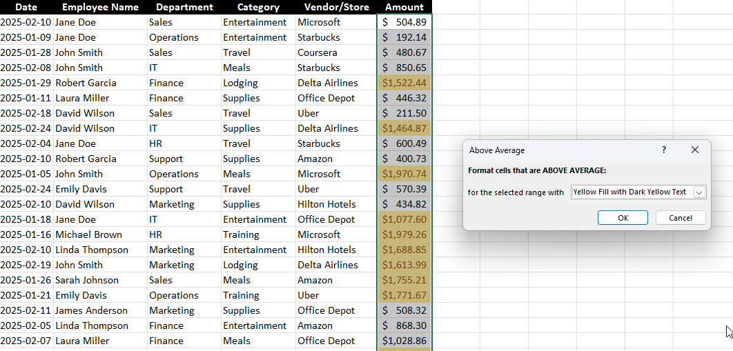
- Above / Below Average: This highlights values above or below the dataset’s average. Below, all the values that are above average are highlighted in yellow. Here again, there’s no need to actually calculate what that cutoff point is. Excel determines the average and then highlights the values that are over that.
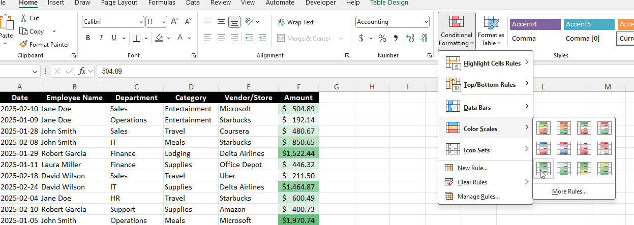
Data Bars, Color Scales, and Icon Sets
These options provide a graphical representation of data, and they can be a more powerful way to visualize your numbers.
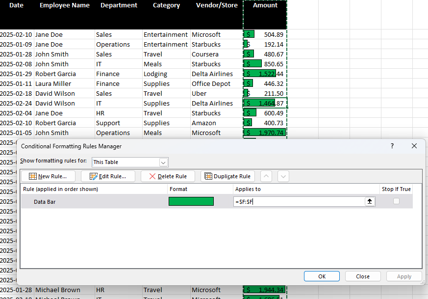
- Data Bars: Fill the cell with a bar proportional to its value. And with this conditional formatting, it’s easy to spot high and low values in relation to one another.
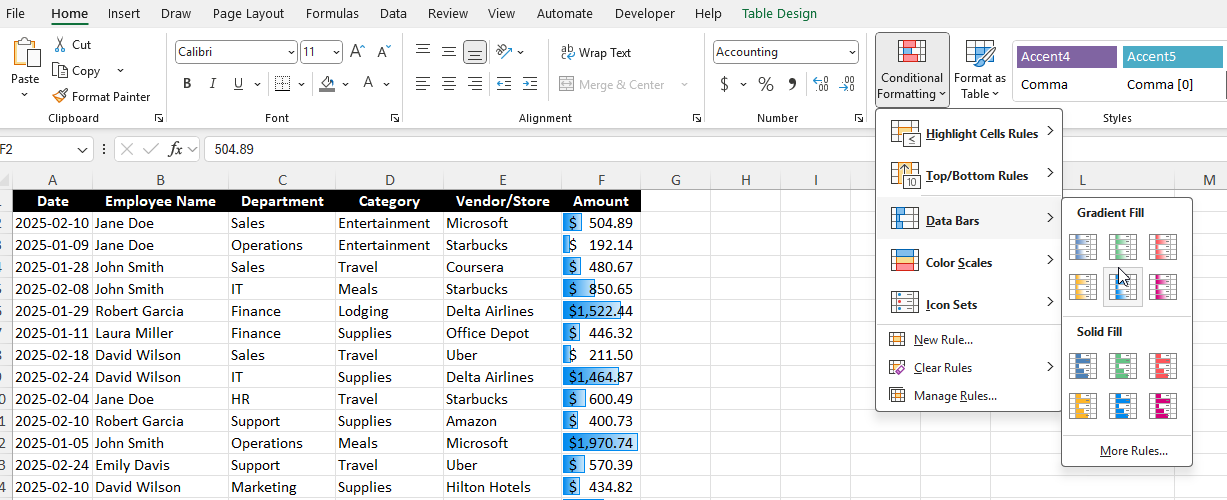
- Color Scales: Apply a gradient of colors based on value distribution. You can use three different colors, or you can use shades of a color, where larger values will appear darker while smaller ones will be lighter in color.
- Icon Sets: Display different icons (arrows, checkmarks, etc.) based on value thresholds. This does a similar job as the other options, but now you can utilize icons instead of just colors.
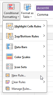
Creating your own rules
The pre-defined conditional formatting options can be useful, but you may prefer to make your own. By doing so, you can apply more customization to your rules. If you skip pass the first options on the conditional formatting menu, you’ll see an option to create a New Rule:
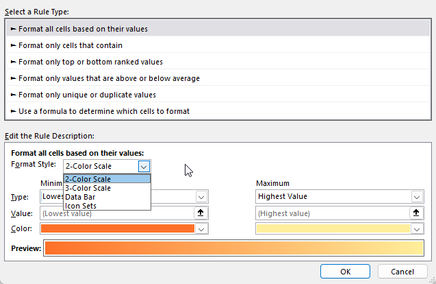
From here, you’ll get similar options as to the pre-defined ones, including formatting them based on their values, top or bottom rankings, above or below average, and so on.
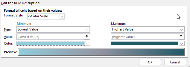
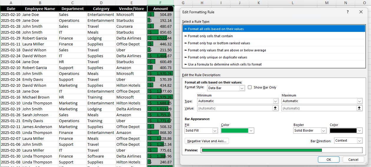
Formatting cells based on their values
For this rule, you can specify the type of color scale you want to use (2 colors, 3 colors, data bars, or icons)
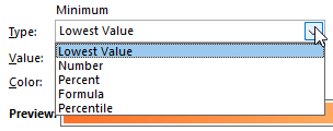
You can also change how the minimum and maximum values are determined, whether they are based on simply the lowest value in the range, a specific number, a percentage, formula, or percentile.
And you can also change the color scheme, to determine how you want the gradient to look, and how it will progress from the minimum to the maximum. By changing the drop downs, below I’ve changed the gradient to go from a light teal to a dark teal color.
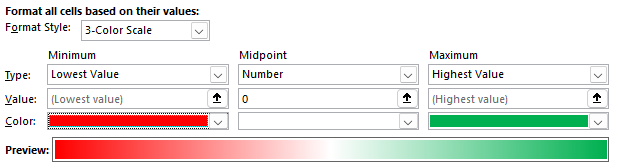
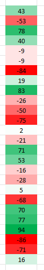
If you select a 3-color scale, you’ll notice you’ll also have a midpoint option, where you can have a third color. If you’re dealing with values that are positive and negative, you may want to use a 0 value for the midpoint and make the color white. This is how I’d set it up for high and low values when there are negatives. The largest negative values will be in red and the highest positive values will be green, while anything close to 0 will be white.
Here’s how this would look on a range of values between -100 and +100:
If you select a data bar as your option, you’ll notice different settings for that. Not only can you specify the minimum and maximum values, but you can also adjust the appearance of the bar:
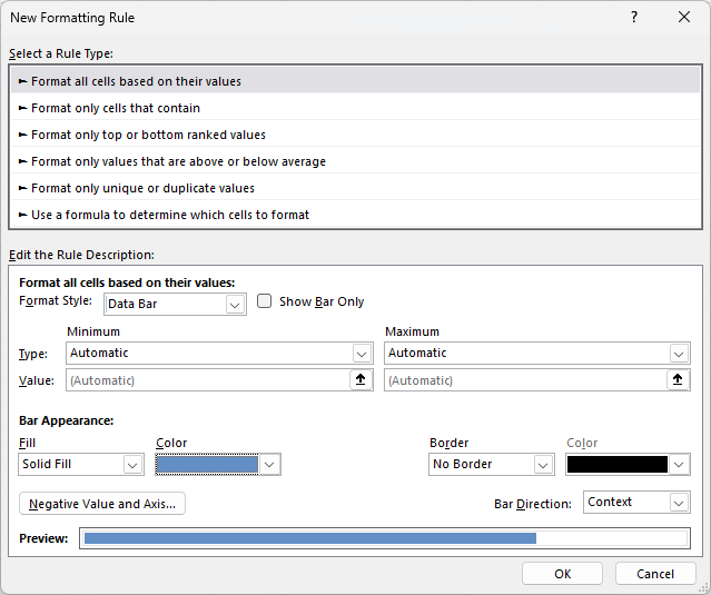
In the below example, I’ve modified the data bar so that it is green with a black solid border:
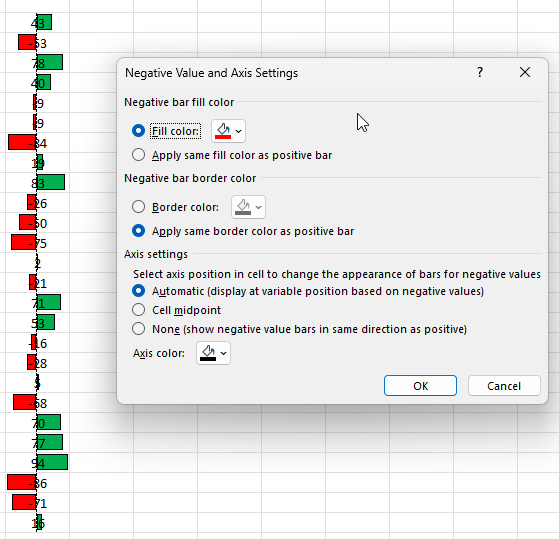
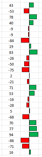
If you have negative values, you can click on the Negative Value and Axis to modify how those values will show. By default, if they are negative, the fill color is set to red, but this too can be changed.
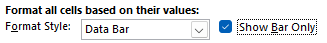
TIP: If you don’t like the look of the above formatting because it looks messy, consider copying the values in the next column. Then, create the same conditional formatting rules but select the option to Show Bar Only next to the Data Bar option:
By doing this, you can have your values in one column, and then just the bar in the other column. When you show just the bar only, it doesn’t display the values anymore. In the below example, the values are in both columns, but with this formatting applied, they are no longer visible in the column on the right.
If you create a new rule using icon sets, you’ll get yet a different set of options:
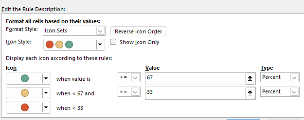
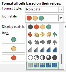
There are many different types of icons you can choose from, allowing you to be creative in how you want the formatting to be applied.
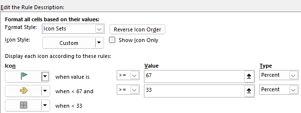
However, you can still mix and match. You aren’t locked into a specific set of icons. You can change the look of each icon by clicking on the drop-down option next to it.
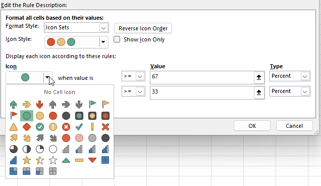
Below, I’ve used a mix of various icons that don’t conform to any pre-defined style:
Although the default is to use a percent, you can also change this to formatting a value based on its numerical value, a formula, or a percentile.

Format only cells that contain certain values or text
This next section is a bit simpler in that there are fewer options. You specify how you want to format them based on what they contain, and if they meet a certain criteria:
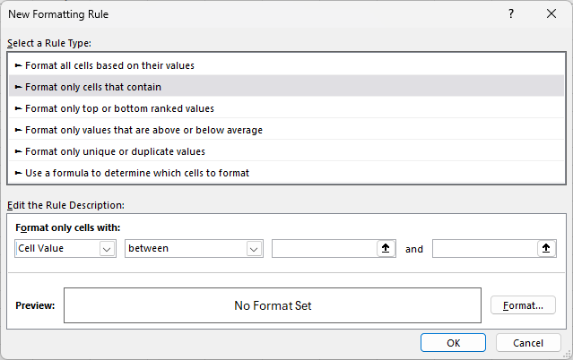
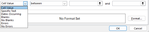
For the first drop-down option, you can specify if you’re looking for a certain value, text, date, or whether it’s a blank or error.
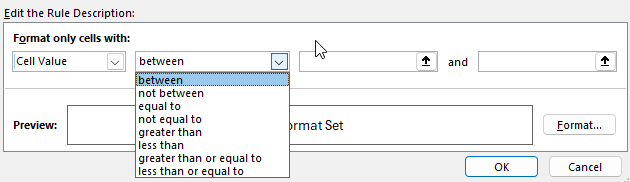
Depending on what you select, the next drop-down option may change. But if you leave it to the default cell value, then you can also specify whether it’s within a range of values, greater than, equal to, or less than a certain value.
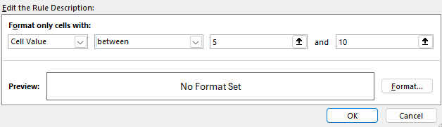
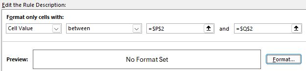
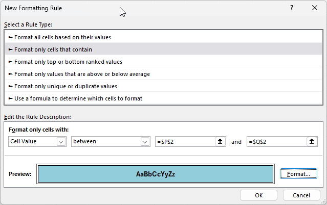
Since I’ve selected between, I need to enter multiple values, one being the start of the range and the other being the end. In the below example, I’m looking at values that are between 5 and 10.
TIP: Anytime you see the up arrows, that means you can specify a certain cell to link the rule to. And when you do so, your rule becomes dynamic. As the value changes in the cell that you’ve specified, the formatting rule will update. This can be helpful because you can easily change the value without having to go into the conditional formatting settings.
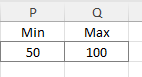
In the example below, I’m no longer specifying exact values but instead referencing ranges, P2 and Q2:
In my spreadsheet, I can setup these cells accordingly, so that I know they are my min and max values for my conditional formatting rule:
But before any conditional formatting gets applied, I need to specify the formatting I want. Since I’m creating a rule type from scratch and not relying on pre-defined rules, I also have to set my formatting. To do this, I need to click on the Format button, which opens up the Format Cells options. And just like when you’re formatting cells in Excel, you can specify how you want the cell to look, including its font style, number formatting, border, and fill color.
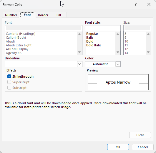
In my example, I’ve created the rule so that it will apply a blue fill color, with a solid black outline, and bolded black text.
This is how it has been applied to my range of values:
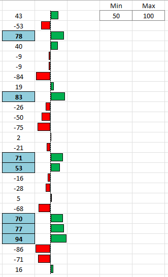
Format only top or bottom ranked values
This rule type is an even simpler one since we are only looking at the largest or smallest values. The first drop-down option allows you to choose from either Top or Bottom.
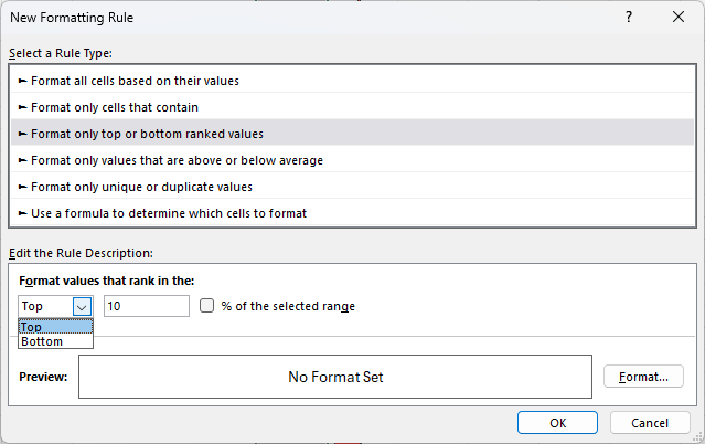
The next field is where you specify the number of items. If I leave it to 10, then it will grab the 10 largest items in the range I’ve selected. But if I check off the option to say % of the selected range, then it will grab the top 10% of the values. For example, if in my range I select 26 values, it will highlight only the two largest values since that will mark the top largest ones, based on the size of the range. Here’s the difference in the two approaches:
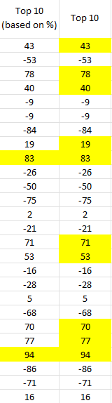
Format only values that are above or below average
This option is similar to the one in the pre-defined conditional formatting rules. However, you have a bit more flexibility here in being able to also format them based on how many standard deviations they are away from the average.
You will also need to set the formatting you want to apply. You could create one rule for if something is 1 standard deviation away and another one for if it is 2 standard deviations, etc.
Format only unique or duplicate values
With this option, there are the fewest choices to select from. You can either highlight duplicate values or unique values. And as is the case with other conditional formatting rules you create from scratch, you also have to specify your own formatting.

Using Formulas in Conditional Formatting
The last section is the one which can allow for the most customization. Here, you can create your own custom formulas. This allows dynamic formatting based on complex conditions.
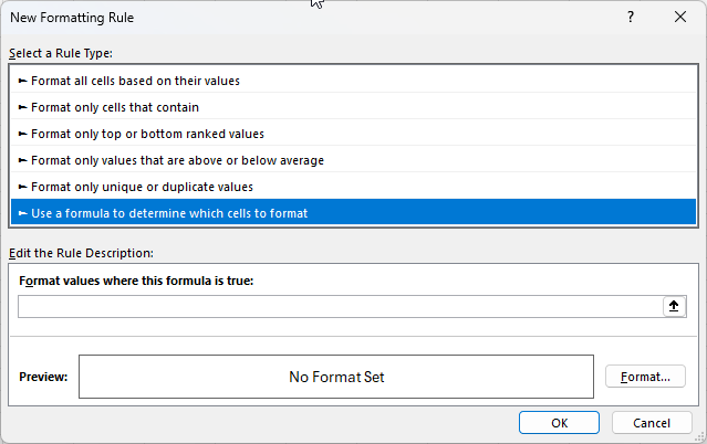
The key thing to remember is that you want the formula result to be either a TRUE or a FALSE value in the end. That will determine whether the criteria is met. A good strategy here is to set up your formulas first in your spreadsheet, and then copy them into the conditional formatting formula. Follow this guide to setup advanced conditional formatting rules like a pro.
Here’s a quick overview of what you can do:
- Highlight Cells Based on Another Cell’s Value.
- To highlight cells in column B if the corresponding cell in column A is greater than 100: =A1>100
- Highlight Even Rows for Better Readability
- To apply formatting to alternating rows (like zebra striping): =MOD(ROW(),2)=0
- Highlighting Expired Dates
- To highlight dates in column A that are past today’s date: =A1<TODAY()
- Highlight Cells Based on Text Values
- To highlight all cells in column A that contain the word “urgent”: =SEARCH(“urgent”, A1)
- Make Non-Zero Values Stand Out
- You can make zero values invisible or light grey to make them less prominent in your sheet, allowing other values to stand out more.
These are just a few examples of what you can do with formulas but you have many more options with this approach.
Common issues with conditional formatting rules in Excel
Here are some of the most common issues you may encounter when creating conditional formatting rules in Excel.
Why are my conditional formatting rules being applied to the wrong cells?
This can happen for a couple of reasons. The first is that you haven’t selected the correct range when setting up your rule. If you go into the Conditional Formatting menu and select Manage Rules, you will see all the ones that are applicable (to your current selection).
The current rule here applies to all the cells in column F. If I need to change that, I can either edit right within the Applies to box or I can click on the up arrow and select the range manually.
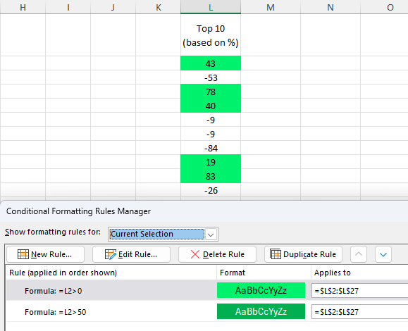
Another issue related to ranges can happen when there is a problem with the cells your formula is referencing. Take a look at the screenshot below and see if you can figure out why the formatting isn’t correctly applied. Even though the rule is simple and is just looking at whether the cell’s value is greater than 50, it is being applied to the wrong cells.
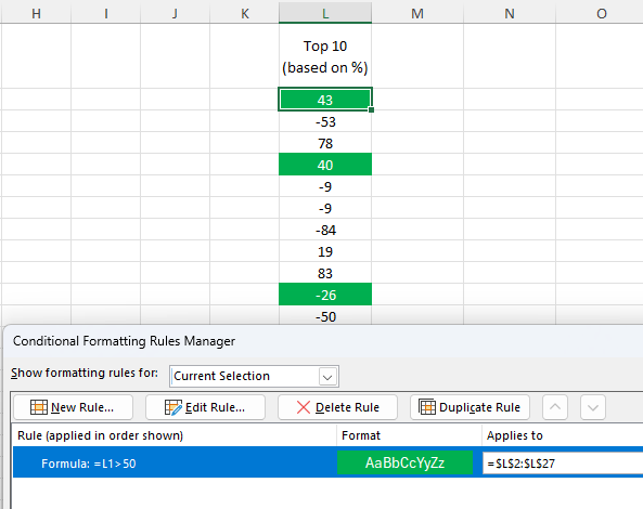
Although the column is correct, the problem is the range. Notice that the rule is L1>50 but it is being applied to $L$2:$L$27. The first cell is off by 1 row, so the formula will always be offset by 1 row. That means that when it’s evaluating L2, it will look at L1. And when it is looking at L3, it is looking at L2. In the above example, because there is a text value it is not a number and thus meets the criteria. And the value of 40 is highlighted because the formula is looking at the value above it (78).
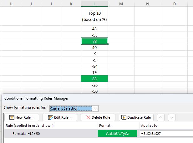
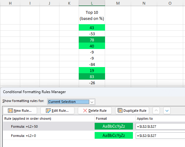
If I modify the formula so that it is changed to L2>50, now the conditional formatting is applied correctly.
The rules won’t update, however, until you click the Apply button. This is necessary to do anytime you make changes to a conditional formatting rule.
Why are the wrong conditional formatting rules being applied?
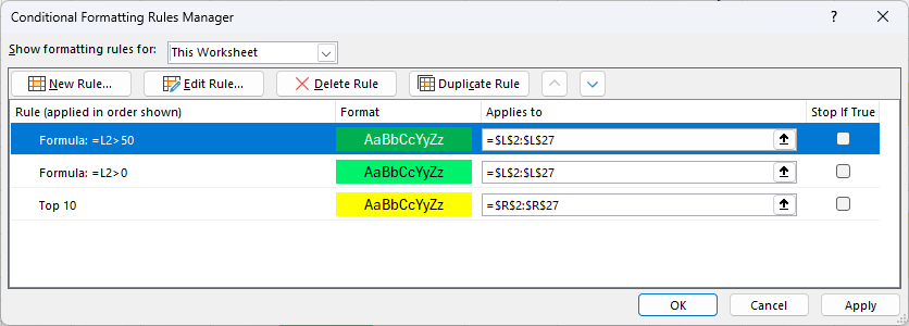
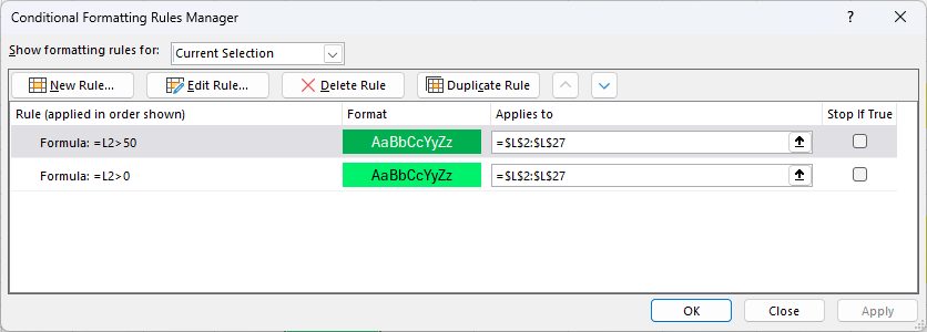
If you have multiple conditional formatting rules in place, you may encounter an issue where the wrong ones are being applied. Consider the below example, where I have created a rule when a value is greater than 0 to be highlighted light green, and another one so that it is dark green when it is greater than 50.
Since a cell can meet both criteria and be both higher than 50 and 0, it’s important to prioritize the rules correctly. To fix this issue, I need to select the bottom rule, and click on the up arrow to push it to the top. After doing this, and clicking apply, the values over 50 are filled in with the darker green color.
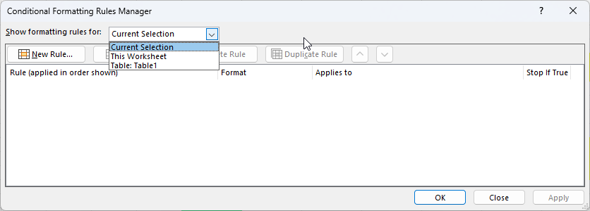
Why am I not able to find my conditional formatting rule?
If you’ve created a conditional formatting rule but can’t find it, it’s likely that you’ve selected a cell it isn’t applied to. If you go to the Conditional Formatting menu and select Mange Rules, you’ll see all the rules that you’ve created. But by default, this shows the rules that are applied to your current selection. You can, however, change the drop-down option to show rules for the entire sheet and anywhere else there are rules setup:
After changing it to This Worksheet, I now see all the rules that I’ve created on the worksheet.
How do I delete a conditional formatting rule?
In some cases, you may find that you have too many conditional formatting rules and want to get rid of some. In this case, go back to the conditional formatting rules manager where you’ll see a list of all the rules you have created.
From here, you can select any rules that you don’t need anymore, and click on the option to Delete Rule. Be sure to click on Apply afterwards to make sure your changes go into effect.
If you liked this post on How to Create Conditional Formatting Rules in Excel: The Ultimate Guide, please give this site a like on Facebook and also be sure to check out some of the many templates that we have available for download. You can also follow me on Twitter and YouTube. Also, please consider buying me a coffee if you find my website helpful and would like to support it.