Dynamically Filter Data Using Only a Formula

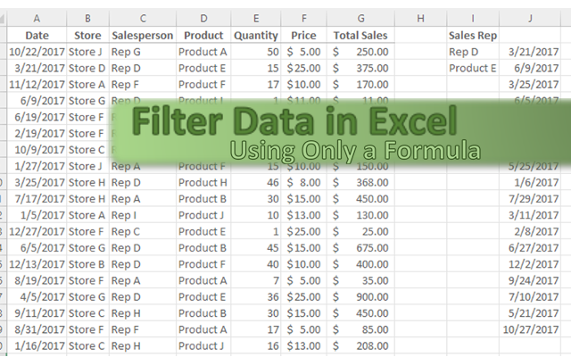
In my previous post I went over advanced filters in Excel. This time around I’ll go over how to achieve the same result using just a formula. No macros, no VBA, just through a not-so-simple formula that can dynamically update based on your selections.

I’m again going to use my sample database file for this example. Here’s an excerpt of what that looks like:

Filtering based on one criteria

I’m going to start by filtering all that entries for a specific sales rep.

First, I’m going to use the INDEX function to select the range from where I’m pulling data from.

=INDEX(SampleDatabase!$A$1:$G$1000

For my results, I’m going to want them to show up in the order they appear in the database. For example, in the excerpt above Rep D shows up on lines 3 and 5, and I want that same order to stay intact.

In order to do this, I’m going to use the IF, SMALL and ROW functions, which will be inserted in the INDEX function.

SMALL(IF(SampleDatabase!$C$1:$C$1000=$I$2,ROW(SampleDatabase!$A$1:$A$1000),””),ROW(A1)),1)

$C$1:$C$1000=$I$2 : In this argument, assume that $I$2 is where I have my sales rep name, in this case it would be Rep D. Because I’m only interested in rows that relate to Rep D, this is the main argument that I want to evaluate.

ROW(SampleDatabase!$A$1:$A$1000), “”) : This will return the row number if the above argument is true. It doesn’t matter whether I reference column A, B, C or any other since I’m only pulling the row number. If it isn’t a match, the result will be a blank value.

ROW(A1) : This returns a value of 1, and what this will accomplish is that it will pull the smallest row number from the above list. For instance, for Rep D we know that lines 3 and 5 will be a match, but the smallest number, or the first time that there is a match, is 3. As I drag this formula onto subsequent lines, the row number, because it isn’t frozen, will change and on line 2 it will pull the second smallest row number, on the third line it will be the third smallest, and so on.

The last argument is which column you want to extract. I left it as 1, and that will return the date since that is the first column in my INDEX argument. However, if I wanted to pull the total sales, I could change that to 7, since that would indicate column G, which is the seventh column in the data set that I specified.

The completed formula will look as follows:

=INDEX(SampleDatabase!$A$1:$G$1000,SMALL(IF(SampleDatabase!$C$1:$C$1000=$I$2,ROW(SampleDatabase!$A$1:$A$1000),””),ROW(A1)),1)

This formula will need to be entered as an array, so be sure to hit CTRL+SHIFT+ENTER.

The first five results look as follows:

The one caveat is that if you don’t know how many entries you’ll have and copy the formula down too far, you’ll inevitably end up with #NUM! errors because the formula has not found any more matches. What you can do in this case is use the IFERROR function and include it in the formula:

=IFERROR(INDEX(SampleDatabase!$A$1:$G$1000,SMALL(IF(SampleDatabase!$C$1:$C$1000=$I$2,ROW(SampleDatabase!$A$1:$A$1000),””),ROW(A1)),1),””)

What this will do is now show a blank value if there are no more matches.

Filtering for multiple criteria