Color Calculator Template: Sum by Color in Excel

Unless you’re still stuck on old versions of Excel, you probably know that you can filter data using colors. And by doing so you can use the SUBTOTAL function in excel to tabulate those amounts. But in this post, I’m going to show you something a little different. By using a macro, I’ll highlight cells containing values and then sum them by color in Excel, without needing a subtotal or a filter. This free template will just use VBA to populate the totals.

How the template works

In this template, all you need to do is enter your data and then assign whatever formatting you want to use to identify a cell to the corresponding category. As long as a cell has the exact same formatting as the category, it will be included in that category’s calculation.

I got the idea when I was trying to quickly analyze expenses and didn’t want to go through a whole process of putting it into a complex budget template. Rather than setting up logic to classify whether an expense falls into one category or another, I thought color-coding could be another way you could quickly group expenses.

Here’s a quick video showing you the template in action from color-coding cells to calculating the totals:

Setting up the data

In the template, there’s one section dedicated to the raw data where you’ll enter your inputs:

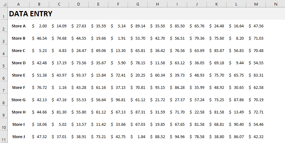
You can input data up until column N, although I’ve left the column blank for a buffer. In this example, I’ve put in random numbers and grouped them based on a store value in column A. This can be all numbers, it doesn’t really matter, I just preferred to have some grouping.

Next to the data entry, I’ve got a list of categories set up in column O:

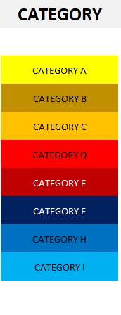
You can add as many categories as you like. How they’re color-coded here is how you’ll need your cells will need to look to ensure they’re in the correct categories. For instance, any cells that are highlighted in light blue will go into Category I. Whereas anything in a dark red will belong to Category E.

You may think this would be a painful process to try and color-code your data based on all these different categories. After all, what if you get the shade wrong or the font color is wrong. The solution’s really simple and you just need to use our trusty friend, the Format Painter. If you’re not familiar with it, this is what it looks like:

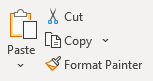
It’s on the left-hand-side of the Home tab where the copy buttons are. What you can do is select the category you want to be assigning data to, click once on the Format Painter and then click on the cell you want to highlight with that exact same formatting.

If you’ve got multiple cells that you want to apply the formatting to and don’t want to keep repeating this exercise, then Double-Click on the Format Painter. You can now continue selecting cells and the Format Painter will take care of the formatting for you. You won’t need to re-select it each time. Once you’re done with the formatting and want to stop applying it, click on the Format Painter again to stop.

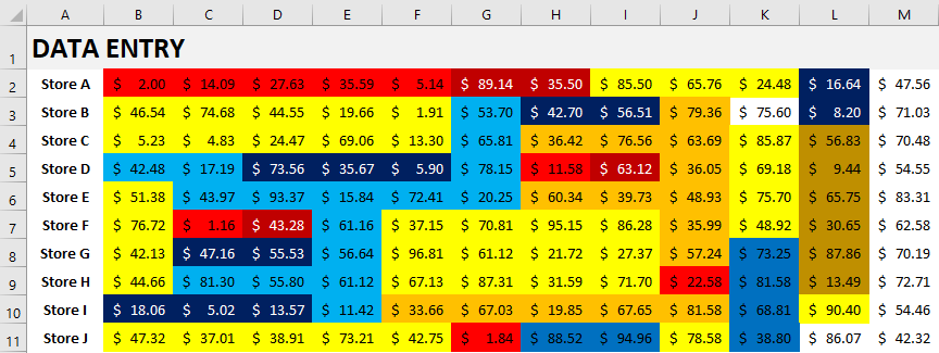
I’ve color-coded some of my data based on the categories, and here’s how it looks:

Updating the calculations

On the right-hand-side of the page there’s a button that says Update. This will update the totals based on the color-coding. You’ll need to have macros enabled for this to work. Above the button you’ll see the total of all the values in columns and how much is unallocated.

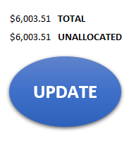
Clicking on the update button will trigger the macro to run the calculations. After pressing the button, here’s what my categories look like and the totals corresponding to their color-coding:

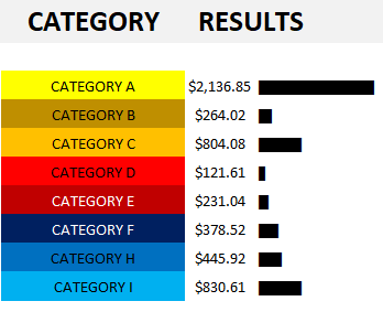
You’ll notice I’ve also created visuals to see the relative size of each category using the REPT function. If you’re interested in learning how to use this function, check out this post.

Anytime you make changes to the color-coding, be sure to hit the Update button. I didn’t want the formulas to update every time there was a change on the sheet because that can sometimes slow a spreadsheet down, especially since it would involve recalculating all the totals.

The code

Here’s the VBA code itself on how the update button works:

Sub Oval1_Click()

Dim clvalue, clcolor As Double
Dim cl, colorrange As Range
Dim lstrow As Integer

lstrow = ActiveCell.SpecialCells(xlLastCell).Row

Set colorrange = Range("colorrange")

'clear data range
colorrange.Offset(0, 1).ClearContents


For Each cl In ActiveSheet.Range("A1:O" & lstrow)

    If IsNumeric(cl) Then
    
        clcolor = cl.Interior.Color
        
            For Each lookupcl In colorrange
    
                If lookupcl.Interior.Color = clcolor Then
                    lookupcl.Offset(0, 1) = lookupcl.Offset(0, 1) + cl.Value
                    GoTo nextcl:
                End If
    
            Next lookupcl
    End If

nextcl:

Next cl

End Sub

There’s a named range called “colorrange” that it cycles through, and those are the categories in column O on the spreadsheet.

Using the template

This isn’t a terribly complex template to use. However, it can help if you want to quickly group items. It’s a unique way to classify expenses rather than just using drop-downs and complicated formulas. And it makes it easy to sum data by color in excel. The way I found it useful was to list your vendors or stores in column A. Then, arrange transactions by date (e.g. the first transaction is in column B, then C, and so on). But this can be used in a variety of different purposes to help classify data.

If you want to reset the calculations, just change the data back to the default formatting or something that doesn’t correspond to a category you already have, and then click update.

Download

The template is free to download and it’s available here.

If you liked this post on how to sum by color in Excel, please give this site a like on Facebook and also be sure to check out some of the many templates that we have available for download. You can also follow us on Twitter and YouTube.