How to Create a Named Range in Excel

Naming ranges offers an easy way to refer to a single cell or range without having to remember the address, and instead referring to it by name instead. This comes particularly useful if you will continually be referring to that cell. 

– Less time consuming to find a named cell

– Easier to put into formulas

– Easier to reference in VBA

– Easily inserting hyperlinks in documents

Below I have sales data listed by month. If I wanted to reference total sales I would need to refer to cell B14.

Let’s say this sheet is just one of many, and these are sales for product A.  The more products I have, the more useful it becomes to have named ranges, otherwise I would have to either a) remember the location when typing a formula, or b) navigating to the cell I want to reference. By using a name, it is easier to recall and doesn’t take much effort to include in a complex formula that may include many references.What I could do is name cell B14 as ProductASales (and subsequent ones could follow the same patter – ProductBSales, ProductCSales, etc..)

All I do is select cell B14 and type ProductASales in the cell reference that previously had B14. B14 still exists, but now I can reference the cell by just typing in ProductASales as well.

A range can have more than one name. If you want to delete or edit a name select the Name Managerunder the Formulas tab

I find that I have created two names for the same range. To delete one I just select the name I don’t want and click Delete. Now if I just wanted to change the range I can click Edit

There I can change the range to whatever I want.

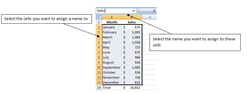
Named ranges can also be used for multiple cells in the same way.

Note that a named range will move as a relative reference. If you insert or delete rows the name will move along with your cells. It can also expand, just like any other range in Excel. If for instance you insert a row between May and June, that will add that row to the range. Instead of including the cells from A2:B13, it will now include the cells from A2:B14 – since December will be pushed down to row 14.

Now that the ranges are setup, they can be referred to in a formula.

This won’t work the same way for the Sales range since it relates to more than one cell. However, I can use it as part of a formula, vlookup for example:

Here I am using Sales as a table. Instead of typing out the full range A2:B13 I only have to type in Sales.

But let’s say you didn’t realize you could use named ranges and have been manually entering the ranges. You can update your formulas so they reflect the named ranges by doing the following:

Under the Formulastab, select Define Name, and Apply Names.

 At the following screen I select both names and press OK.

Now all my formulas with B14 or A2:B13 will be replaced with ProductASales, and Sales, respectively. This won’t affect your formulas in any way but now if you look at a formula you can easily see if it is referencing a named range.

Another benefit of using named ranges is that it makes it easier to keep formulas consistent. In VBA, to reference these ranges, unnamed, would be as follows:

Worksheets(“Sheet1”).Range(“B14”)

Worksheets(“Sheet1”).Range(“A2:B13”)

The problem with this is that if you move the cells around, cut, copy, the references in VBA are absolute and will never update the way relative references in Excel will.  However, if you use named ranges, this problem is avoided. The reference would be as follows:

Range(“ProductASales”)

Range(“Sales”)

If you are coding in another worksheet, you will have to qualify which spreadsheet the named range is in:

Worksheets(“Sheet1”).Range(“ProductASales”)

Worksheets(“Sheet1”).Range(“Sales”)

Now if these ranges are moved within Excel, you don’t have to worry about updating them within VBA.

By using a named range you can also easily add hyperlinks into your spreadsheet. For example, let’s say on Sheet 2 I want to link to the sales data:

On the Insert tab, select Hyperlink.

Select Place in this Document and you will see a list of the defined names. If I press Sales and click OK this will create a hyperlink in the active cell:

Now if I click on the Sales link in cell D6 it will bring me to the named range that belongs to Sales.