2 Excel Functions That Can Eliminate the Need for an Amortization Table

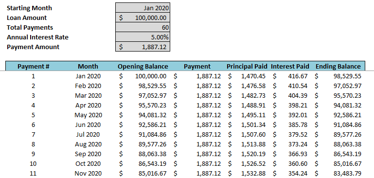
An amortization table is a useful tool when you need to calculate interest payments, principal payments, and to track the balance that’s owed on a loan. However, you don’t have to create a full schedule to get these values and below I’ll show you two functions that can get you that information quickly and easily. First, let’s start with what a typical amortization schedule looks like.

Creating the amortization schedule

When you set up an amortization schedule, you’ll track the balances, interest, and principal payments. It often looks something like this:

You could use the table to determine what the balance is at the end of period 10 or to add up all the interest payments up until that point. However, there’s another way to arrive at those totals, and that’s using two functions that are available in the newest version of Excel: CUMIPMT and CUMPRINC.

Using the functions

In the amortization schedule, we can see that the ending balance of the $100,000 loan by the end of period 10 is $85,016.67. We can use the CUMPRINC function get to that total as well. The function takes on the following arguments:

To calculate the cumulative principal payments, I’ll enter the formula with the following arguments:

=CUMPRINC(0.05/12,60,100000,1,10,0)

This gives me a total of -$14,983.36. When added to $100,000, it nets out to a balance of $85,016.64 — within just a few cents of the amount on the amortization table. The function gives you the flexibility to specify which periods you want to extract and so you aren’t limited in just tabulating the totals for the first 10 periods or starting from the beginning. You can start from period 13, or the second year, and so on.

If you want to calculate the total interest payments, then that’s where you can use the CUMIPMT function. It has the same arguments as the CUMPRINC calculation, so the formula will look very similar to what’s above:

=CUMIPMT(0.05/12,60,100000,1,10,0)

This tells me that the cumulative interest payments during the first 10 payment periods is $3,887.87. This matches what I would get by adding the interest payments in my amortization table over the same period, this time to the penny.

Should you use these functions instead of an amortization table?

On older versions of Excel, you won’t have access to these functions but if you’re using Microsoft 365 or Excel 2019, then these functions are available and can potentially serve as replacements for an amortization table. Now, if you need the table for audit purposes it may not be possible for you to do without an amortization table completely. But if you’re only generating the table just to determine how much you’ve spent on interest or what your balance will be at some point in the future, then these functions can certainly replace doing a full-blown amortization table.

If you liked this post on 2 Excel functions that can eliminate the need for an amortization table, please give this site a like on Facebook and also be sure to check out some of the many templates that we have available for download. You can also follow us on Twitter and YouTube.