Historical Stock Returns by Month

Have you ever wondered how a stock has typically performed month over month? Using a spreadsheet, you can calculate monthly returns and identify patterns of which months are traditionally strong for a stock, and which ones aren’t. In this example, I’m going to use Google Sheets to pull in stock prices and calculate historical stock returns by month.

Start with pulling in historical stock prices

To get started, I’ll need to extract a stock’s price history. This can be done using Google Sheets’ GOOGLEFINANCE function. The key is in setting a start date that goes far enough back to ensure you get enough historical data to use in your calculations. A good function to use within that is the TODAY() function which ensures you will always be counting backward from today’s date and don’t need to hardcode a date. If I want to go back to 2008, for example, I can set my formula to deduct about 5,000 days.

To pull Amazon’s stock price going back that far, this is what my formula would look like in Google Sheets:

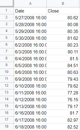
=GOOGLEFINANCE("AMZN","price",TODAY()-5000,TODAY())

Now I have the following values:

The one problem here is that the date values contain the time, 16:00:00, which represents the 4 pm closing time of the stock market. I only want the actual date since I’m going to be doing a lookup and don’t want to include time. To extract just the date, I can use the DATE() function and use the YEAR(), MONTH() and DAY() functions to refer back to the values in column A. For example:

=DATE(YEAR(A2),MONTH(A2),DAY(A2))

The above formula would give me the date in column A without the time. I’ll add an IF statement at the start so that in case the value in column A is blank, my formula simply won’t compute anything:

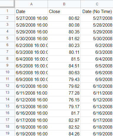
=if(A2="","",DATE(YEAR(A2),MONTH(A2),DAY(A2)))

Now I have a table that has just date values without any time:

Creating a date matrix

Next, what I’m going to do is create a matrix that has years going vertically and months going across:

I’m going to fill in these values with the stock’s returns in each of those months. The key to making this work is by using the DATEVALUE() function which allows me to enter a date. For example, if I entered the following formula:

=DATEVALUE("Jan 1, 2022")

It would result in the following output:

1/1/2022

In the first cell of my matrix, for the JAN 2021, I’ll combine the month abbreviation (JAN) with the year (2021) and the first day (1). Here’s how that would work if the month name is in cell F1 and the year is in E2:

=DATEVALUE(F$1&" 1, "&$E2)

However, let’s assume I don’t want to pull the first day of the month and instead want to pull the ending month’s value. For that, I can use the EOMONTH() function. And then I would enclose the current formula within that:

=EOMONTH(DATEVALUE(F$1&" 1, "&$E2),0)

The 0 value at the end indicates how many months I want to jump by. And since I just want the end of the current month, I don’t need to jump by any months, which is why I set it to 0. At this point, I have a date, and now I can use this inside of a MATCH() function to find the row that matches this date. Assuming the date values in are column C, here is the formula:

=MATCH(EOMONTH(DATEVALUE(F$1&" 1, "&$E2),0),$C:$C,1)

And lastly, inside of an INDEX function that will return the corresponding price from column B:

=INDEX($B:$B,MATCH(EOMONTH(DATEVALUE(F$1&" 1, "&$E2),0),$C:$C,1),1)

Now the formula will pull in the price for a given month. But if I want the month-over-month return, I need to take the month-end price and divide it by the previous month’s ending value. To get the previous month’s price, I use the same formula except instead of a 0, I’ll enter -1 for the number of months:

=INDEX($B:$B,MATCH(EOMONTH(DATEVALUE(F$1&" 1, "&$E2),-1),$C:$C,1),1)

I’ll combine the two formulas now, taking the current month-end price and dividing it by the previous month’s value and also deduct -1 at the end to adjust for it being a percent-change calculation:

=INDEX($B:$B,MATCH(EOMONTH(DATEVALUE(F$1&" 1, "&$E2),0),$C:$C,1),1)/INDEX($B:$B,MATCH(EOMONTH(DATEVALUE(F$1&" 1, "&$E2),-1),$C:$C,1),1)-1

Now, copying this formula across the entire matrix, I can see the stock’s historical returns by month. I’ve added some conditional formatting to contrast the good months from the bad ones:

Besides relying on colors, I can also add a win rate % where I can count the times where the return was more than 0% (i.e. a ‘win’) and divide this by the total number of values. In column F, for January, the formula looks like this:

=COUNTIF(F2:F12,">0")/COUNTA(F2:F12)

I’ll also average the returns so that it’s easier to see the best and worst-performing months:

Judging from this, April looks to be the best time to own Amazon’s stock. It normally returns a positive return and its average over the past 11 years has been a gain of just under 8.5%. To re-create this analysis for other stocks, simply change the ticker symbol.

If you liked this post on How to Calculate Historical Stock Returns by Month, please give this site a like on Facebook and also be sure to check out some of the many templates that we have available for download. You can also follow us on Twitter and YouTube.