Want to show your data in reverse order, and want to do so without having to sort it? Using just a formula, you can change the way your data looks. Instead of going from oldest to newest, you can display it from newest to oldest. And you don’t have to alter your existing data set to do it. In this post, I’ll show you can how can flip your data through just a single formula.
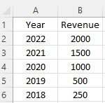
In the below example, I have data going in descending order by year.

If I wanted to change the order so that it’s in ascending order, I could use the sort button. But what if you needed to keep the data the way it is and I just wanted to put in different order, say for the sake of a chart or report. I can accomplish this using the functions INDEX, ROW, and COUNTA. Here’s how it works.
Creating the formula to flip data
The first function I’m going to use is the INDEX function. This is important because this function will include all the data that I need. Since my data is in the range A1:B6, I’ll start with a formula to get the years in column A and reverse them. The formula will start as follows
=INDEX(A$1:A$6
I’m freezing the row numbers because I want to ultimately copy this formula over to the revenue column, and flip those values as well. In the next part of my formula, I will need to grab a count of the values in my range. This can be achieved by using the COUNTA function:
=INDEX(A$1:A$6,COUNTA(A$1:A$6)
The above formula would grab the last value in the range. And while that’s technically what I want, the formula wouldn’t work if I were to copy it down. Thus, I need to add a 1 to it and I also need a way to also deduct 1 — for the first instance, anyway. To make it dynamic, I’m going to use the ROW function.
=INDEX(A$1:A$6,COUNTA(A$1:A$6)+1-ROW(A1))
How this works is that the formula will grab a count of the rows in the data set. Then the formula will add 1 but it will also deduct 1 using the ROW function. In this first formula, my value will be 6 — the same as the count of cells. However, if I drag it down, the formula for the next cell will be as follows:
=INDEX(A$1:A$6,COUNTA(A$1:A$6)+1-ROW(A2))
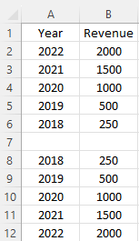
In the above formula, I’ll now be deducting 2 since the row value of A2 is 2. In this case, the row value I will be extracting is 5. The COUNTA function returns value of 6, then 1 is added, and the ROW function deducts 2. By dragging this formula down, it will now continue going backwards and so that the last value will be the first row. If I also copy this over to column B for revenue, I will now have both columns flipped and going in the opposite direction:

If you liked this post on How to Flip Your Data in Excel Without Sorting, please give this site a like on Facebook and also be sure to check out some of the many templates that we have available for download. You can also follow us on Twitter and YouTube.

