

Do you need to create weekly sales reports that compare the same days of the week? This kind of analysis can be tricky to ensure that you are comparing the same day of the week against the same week in the previous year. Simply comparing dates may not be sufficient, as you could end up comparing a Sunday’s revenue numbers against a Friday’s, and depending on the industry you are in, the results could look drastically different. In this post, I’ll show you how you can make reliable comparisons which look at the same weeks and the same days of the week.
Preparing the data
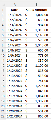
Let’s start with a pretty simple data set which just has the date and the sales amount, as such:
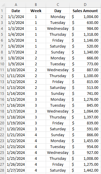
The data set contains sales for January and February of 2024 and 2023. To facilitate the comparisons, I’m going to add fields for the week # and the day of the week. For the week, I can use the WEEKNUM function, which just takes the date as a single argument. And for the day of the week, I’ll use the TEXT function, which can use the “dddd” format type to specify the day. Here’s how the data looks after I’ve added those fields:
Loading the data into a Pivot Table
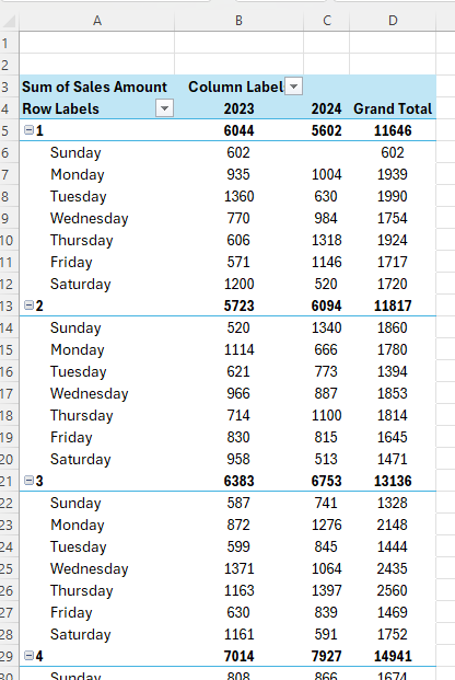
Now that my data is ready to analyze, I can create a pivot table. While any cell on the data set is selected, I’ll click on the Insert tab and select Pivot Table. Next, I’m going to set up the pivot table as follows:
- Columns: Year
- Rows: Week , Day
- Values: Sales Amount
To get the year to show, I’ll select the Date field and put the Years (Date) value under columns. You could also create a formula in the previous step to calculate the year value based on the date. Here is what my pivot table looks like thus far:
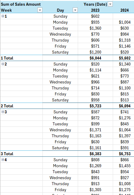
There are a few things I will do improve the appearance and usefulness of the pivot table, including:
- Removing the grand total, since I’m comparing and not adding the values.
- Changing the report layout to a tabular format so that the Week values will now create subtotals.
- Change the value field settings for the Sales Amount so that it resembles a currency format.
Now, I’m ready to do the analysis in the pivot table.
Comparing values in a Pivot Table
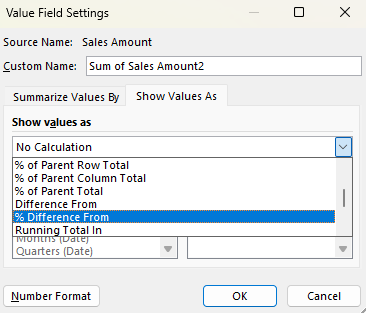
If I want to compare values from one year to the next, I need to pull in another field for the values section. I’m going to pull in the Sales Amount into the section again. While at first, this looks like I’m just duplicating the values, I’m going to change the appearance of the second field. If I click ok the Sum of Sales Amount2 field and select Value Field Settings, I can change how the values are shown. Instead of a sum, when selecting the Show Values As tab, I have the ability to select % Difference From:
I then select my base field. I need to select the Years (Date) field, since I’m comparing years. As for the base item, I’m going to select (previous). If you’re always going to be comparing against a certain year, you can select the specific year. But if you always want to be comparing against the previous year, choose previous.
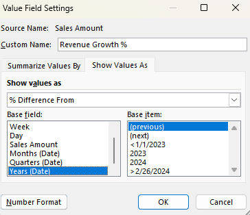
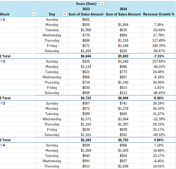
I have also renamed the field to ‘Revenue Growth %’ to signify that the value in the field represents the growth (or decline) compared to the previous year. Here’s how my data looks with the new field:
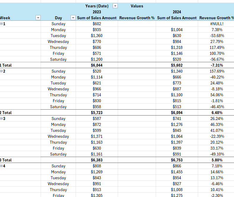
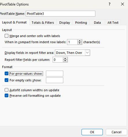
There are a few things I need to fix there. The first is that I have a #NULL! error in the first row. This is because in the previous year, there was no sales, presumably as this would have been a holiday. To fix this, I can go into the Pivot Table options and check off the option For error values show and just leave it blank.
That gets rid of the error. Another thing I need to do is get rid of the unnecessary revenue growth field for 2023. As there is no comparable, it will always be blank for the first year. The simple solution here is to just hide the column entirely. Now I’m left with a pivot table that shows my sales data by week, day, and year, and the year-over-year change in percent:
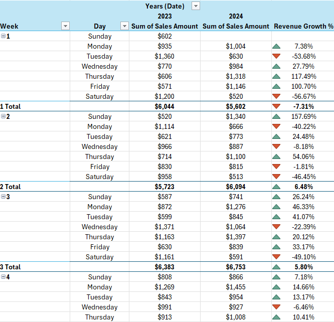
One last thing you may want to do is add some conditional formatting, to help highlight the good and bad weeks and days. Using a directional icon set could help make the results stand out:
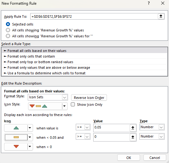
By using this formatting, any values where the growth rate is more than 5%, will have a green triangle. Anything less than 0 will be red, while anything in-between will show a yellow horizontal line.
If you liked this post on How to Compare Weekly Sales in Excel Using a Pivot Table, please give this site a like on Facebook and also be sure to check out some of the many templates that we have available for download. You can also follow us on Twitter and YouTube.