How to Alternate Row Color in Excel

Looking at numbers on a plain white spreadsheet can sometimes make it difficult to differentiate one row from another, especially from afar. It can also make the spreadsheet look a bit bland. That’s why in this post I’ll show you how in Excel you can alternate the color of both rows and columns.

The first step is to create a new conditional formatting rule in Excel

Ultimately, all you need to alternate the row color in an Excel spreadsheet is a little bit of conditional formatting. It just comes down to getting the logic and the formula right in ensuring that the correct rows are highlighted.

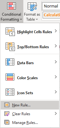
To get things started, select Conditional Formatting from the Home Tab and then Create New Rule

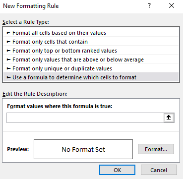
Once there, you’ll want to select the option to Use a formula to determine which cells to format:

This is where we’ll now enter the formula that we’ll want to use for the alternating rows.

Use the MOD function along with ROW to determine which row to apply a different color to

The key function that we’ll need to use is the MOD function. What this function does is it tells us what the remainder is after a number has been divided by a divisor. This is important because what we need the conditional formatting to do is to evaluate each individual row to tell us whether it is an odd or even number, and the MOD function allows us to do that.

For example, the following formula will return a value of 0:

=MOD(6,2)

Since two divided by six will return a result of three and have no remainder, the result of the formula is 0. If, however, we change the formula to this:

=MOD(6,4)

The formula will now return a value of two, since four only goes into six one time, leaving a remainder of two.

Now, it’s simply a matter of applying this logic to each row. To do this, we need to incorporate the ROW function into our formula as well. The end formula is actually not very complex:

=MOD(ROW(),2)=0

The above formula will be true if the row is an even number, and thus, any conditional formatting we have set for that rule will apply. If we wanted to modify every odd row, then the formula could be tweaked as follows:

=MOD(ROW(),2)=1

You could have two sets of rules, one for odd rows and one for evens, but that’s really not necessary. Instead, you can simply select all the rows and then apply the formatting you want for the even rows, and then create a conditional formatting rule for the odd rows. This way, the formatting you apply to the entire sheet will be overwritten by the conditional formatting rules for the odd rows anyway and your original formatting will end up applying only to the even ones.

Applying a different color to the different rows

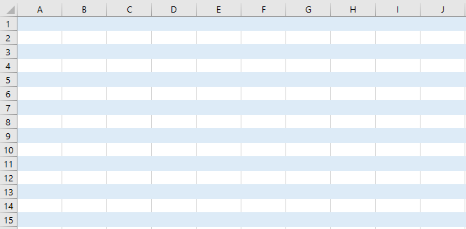
Once you’ve created your rule, then it’s just a matter of selecting the formatting you want to use and how you want to highlight the rows. I’d suggest a color that is light so that you don’t have too much contrast. This is how my Excel spreadsheet looks after applying a light blue color to every alternate row. I’ve left the default formatting in place for the odd rows.

If your spreadsheet doesn’t look like this, check to make sure that you have applied the conditional formatting to the entire sheet and that it isn’t only to a select few rows or cells. If you’re unsure about this, refer back to my earlier post on conditional formatting to help give you a better idea of how it works.

You can highlight alternate columns in a different color too

As you may have guessed, the same logic and conditional formatting rules that we used above can be applied to columns as well. Instead of the ROW function we just need to use the COLUMN function in our formula. That’s really the only difference as the formula will look nearly identical:

=MOD(COLUMN(),2)=1

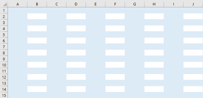
You’ll follow the same steps as far as creating a new conditional formatting rule, but the process is largely the same. The one thing that you’ll notice, however, is that if you have both rules in place, your conditional formatting has now overlapped:

In the above example, the formatting is the same color, but if they were different, the overlap would stand out even more. And that’s where it may take some experimenting with different formats to ensure that you get the right overlap and that the different formatting rules blend well together. Assuming, of course, that you want both rules in place.

Other options to alternate the row and column color in Excel

While this post showed you how to change colors for odd and even rows and columns, you can certainly extend that logic even further. For instance, you could decide to highlight every third row by changing the MOD function so that you’re dividing by three rather than two. As long as the logic is sound, you can modify these formulas so that they alternate the rows that you want.

For example, if you wanted to alternate the color of every fifth row and every 13th row on your Excel spreadsheet, you could create one conditional formatting rule to apply to every fifth row and then another for every 13th one as well. Although putting this into one larger formula is possible, it would a bit cleaner to put them into different rules.

When it comes to conditional formatting, there’s a lot of flexibility in how you can structure how your spreadsheet works. However, you also don’t want to get too carried away and make the spreadsheet too colorful and difficult to read. Otherwise, it may end up defeating the purpose and making your spreadsheet less user-friendly.

If you liked this post on How to Alternate Row Color in Excel, please give this site a like on Facebook and also be sure to check out some of the many templates that we have available for download. You can also follow us on Twitter and YouTube.