Do you ever wonder how much of a return on an investment you would have made if you invested money into a stock or major index? In this post, I’ll show you how you can create a template to calculate those returns in Google Sheets. You can also download the one that I’ve made.
Setting up the inputs
To make a template like this versatile and dynamic, it’s important to create cells for inputs so that the values can easily be updated. One cell should be for the investment amount. Another should be for the index or ticker, and the last option should be for the # of years in the past that you want to look back.
In Google Sheets, if you want to lookup the values for the S&P 500, Nasdaq, or Dow Jones, you’ll need to use the following symbols:
Dow Jones: .DJI
Nasdaq: .IXIC
S&P 500: .INX
There is a period before each symbol. Regular stock symbols, such as GOOG for Alphabet are entered normally without any periods. But for an index, you need to add a period before the symbol. And as you can see from the symbols, they aren’t obvious as the S&P 500 uses INX while for the Nasdaq, it’s IXIC. Rather than entering in these symbols, it may be easier create a lookup list, which you can then use in data validation. For example, I have the list of related values posted in E1:F3
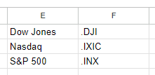
I can then use this lookup so that the user selects Dow Jones, Nasdaq, or S&P 500 and then the corresponding symbol will populate:
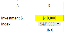
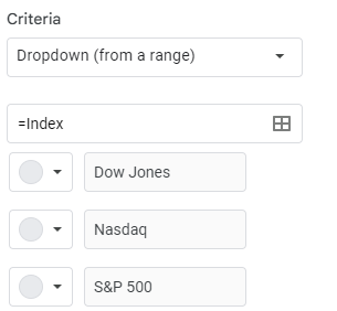
To create a drop-down list in Google Sheets, select a cell and click on Data and press Data Validation. From there, you can either manually enter your options, or you can reference a named range. In my example, I’ve referenced a named range called Index, which holds these values.
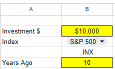
Next, there’s the field for the # of years you want to look back. This will be used in calculating the stock or index’s previous value. That is the final input that I will use for this template:
Calculating the return
To calculate the return from the investment, we need today’s value and the value from the past. To get the current value is simple and just requires the following formula:
=GOOGLEFINANCE(symbol,”price”)
In my file, I’ve created a named range called symbol which relates to the .INX value in the above screenshot. When no dates are entered, the formula will pull in the latest value for the symbol.
To get the previous value takes a bit more work. The formula will start off the same but I need to adjust the date so that it factors in the number of years I want to go back. To do this, I will use the DATE function and specify the year, month, and date values. Assuming I want the exact same date and only adjust the year, here is how I would adjust the formula:
=DATE(YEAR(TODAY())-yearsback,MONTH(TODAY()),DAY(TODAY())
In this formula, yearsback is the named range relating to the # of years I want to go back. In my example, it is set to 10. By adjusting the year argument in the date function by the number of years I want to go back, that will adjust the year and nothing else. The TODAY function returns the current date and acts as a starting point. For the last argument in the GOOGLEFINANCE function I set the value to 1, since I only want the value from a single day.
=GOOGLEFINANCE(symbol,”price”,date(year(today())-yearsback,month(today()),day(today())),1)
The only issue here is that this formula returns a table with headers. To extract just the value, I need to wrap it within an INDEX function:
=INDEX(GOOGLEFINANCE(symbol,”price”,date(year(today())-yearsback,month(today()),day(today())),1),2,2)
The formula will now grab the second row and second column, which relates to the value I want. Now that I have my current previous values, I can calculate the return. For this calculation, I only need to take the current value, divide it by the previous value, and subtract 1:
=currentvalue/previousvalue-1
Here again, I’m using named ranges to easily refer to those values and so it’s easy to see what I’m referencing. The result of this formula is a % change.
Lastly, I need to calculate the value of the investment today. This involves taking the original investment and multiplying it by 1 plus the return. This formula uses named ranges once more:
=originalinvestment*(pctreturn+1)
Here’s what my spreadsheet looks like now when I calculate what a $10,000 investment in the S&P 500 would be worth 10 years ago today:
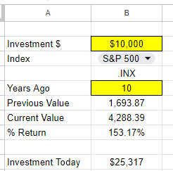
You can see both the % return as well as the dollar amount of that investment. With the cells highlighted in yellow and a drop-down option, it makes it easy to see the fields that can be adjusted. If you prefer to use this calculation for just stocks, you can do away with the lookup and instead just enter the ticker symbol directly. If you’d like to download my version of the template, you can access a copy of it here.
If you liked this post on How Much Money Would You Have if You Invested in the S&P 500 10, 20, and 30 Years Ago, please give this site a like on Facebook and also be sure to check out some of the many templates that we have available for download. You can also follow me on Twitter and YouTube. Also, please consider buying me a coffee if you find my website helpful and would like to support it.

