Calculating and Tracking Streaks with a Custom Function

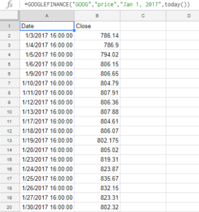
With the stocks markets tanking earlier this month, I thought it’d be interesting to track their historical performance and put into perspective just how badly things have been going lately. For those that don’t know, one of my side jobs is writing articles for the Motley Fool Canada and so naturally this example attracted my interest.

However, there’s not an easy way to calculate this in Excel, and so I decided to go the route of a custom function.

What I’m going to be looking to accomplish is a way to to track how many consecutive trading days that a stock has been up or down, and then also calculate the cumulative value of those gains and losses.

If you’d like to follow along with my example, you can download the file I used here (you’ll have to save the file, open it in Excel and enable content, otherwise you’ll see NAME? errors)

Setting Up the Variables


I want the calculation to start from the bottom (the current cell) and work its way back up, since the latest results will be at the bottom. To do this I create a ‘bottom’ variable that looks like this:

————————————————————————————————————–

bottom = selection.Count + selection.Row – 1

————————————————————————————————————–

I want the user to be able to select what range they want the calculation to apply to, rather than selecting everything.

I also setup a variable for the column, which I named as offsetnum:

————————————————————————————————————–

offsetnum = selection.Column

————————————————————————————————————–

These two variables allow me to set my starting point for my calculation.

Determining if I’m Counting Negatives or Positives

The value of the starting cell will determine if I am going to be looking for positive numbers (gains) or negatives (losses), and so I setup an if statement to determine whether the first value is a gain or loss:

————————————————————————————————————–

If Cells(bottom, offsetnum) < 0 Then
    posneg = “negative”
Else
    posneg = “positive”
End If

————————————————————————————————————–

Start counting


The final step involves counting the values depending on whether I’m looking for positives or negatives:

————————————————————————————————————–

For counter = bottom To 1 Step -1

    If posneg = “negative” Then
 
            If Cells(counter, offsetnum) < 0 Then
                streak = streak – 1
            Else
                Exit For
            End If
         
      Else
   
            If Cells(counter, offsetnum) >= 0 Then
                streak = streak + 1
            Else
                Exit For
            End If
         
        End If
     

Next counter

————————————————————————————————————–

My complete function looks as follows:

————————————————————————————————————–

Function streak(selection As Range)

Application.Volatile
Application.Calculate

Dim bottom, offsetnum As Integer
Dim posneg As String

bottom = selection.Count + selection.Row – 1
offsetnum = selection.Column

‘Determine first value
If Cells(bottom, offsetnum) < 0 Then
    posneg = “negative”
Else
    posneg = “positive”
End If

For counter = bottom To 1 Step -1

    If posneg = “negative” Then
 
            If Cells(counter, offsetnum) < 0 Then
                streak = streak – 1
            Else
                Exit For
            End If
         
      Else
   
            If Cells(counter, offsetnum) >= 0 Then
                streak = streak + 1
            Else
                Exit For
            End If
         
        End If
     

Next counter

End Function

————————————————————————————————————–

Calculating consecutive points gains and losses


Now that I have a function to tell me the current winning or losing streak, I can calculate the cumulative gains and losses.
To do this, I am going to sum as far as the streak goes. And so far starters, I’m going to start with the SUM function. I am also going to use the OFFSET function because I need to determine how many rows up I need to add. The OFFSET will start from the current position and determine how far back I need to go to add up the totals in the current streak.

However, because some streaks are negative, I’ll need to also use the ABS function to just grab the number, regardless of if it is positive or negative. My formula looks like this so far:

=SUM(OFFSET(H2,1-ABS(I2), 0

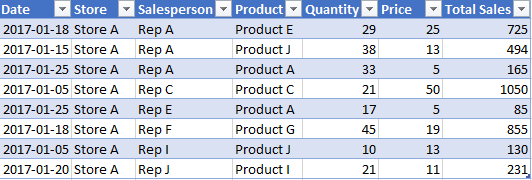
Column H is where my gain or loss value is, while column I is the streak value. Since I want to sum the cumulative gains, I need to reference column H as my starting point.

I added the 1- before the ABS function because that will ensure the number is a negative, meaning that my formula will calculate upward, rather than downward if the number were positive. I also have to decrease the number of cells to offset because I don’t want to include the current cell, otherwise the formula will go too far.

Since I’m not offsetting any columns I set the next argument to 0.

The last argument I need to enter is the height of the offset function, otherwise the formula will just offset by the number specified in the second argument and pull that value, rather than pulling all the values that fall within the range.

This actually involves just copying the same argument again, but this time for the height. My completed formula looks as follows:

=SUM(OFFSET(H2,1-ABS(I2),0,ABS(I2)))

Note

Sometimes with custom functions you might notice that your calculations hang or stop computing correctly. What that means is you just need to recalculate using either F9 or you can edit in the cell and click enter, which will normally trigger a recalculation as well.

Alternatively what you could do is after running the formulas for the dataset, copy them over as values to ensure that they don’t change, since in this case you likely wouldn’t need to recalculate the streak value again.

Creating a Dynamic Dashboard in Excel


Do you want to create a dashboard that will update all of your charts simultaneously based on what filters your users select? Follow the steps below and you can create a professional-looking dashboard without having to use any complex formulas or programming.

Preparing the Data

 
If you have data in Excel that you want to use to create a dashboard, there are a couple of things you’ll want to do first to make sure everything goes well.
 
1. Ensure your data is free of error cells, as this will result in errors.
2. Have proper headings setup so that you know what you are referencing in your dashboard. 
3. Setup a named range for your data, ideally a dynamic one. This will make it easier to link everything to your data quickly and easily.

Making sure your data is clean and ready to go is the most important step, but unfortunately the one that is easily overlooked. After all, if you’re data is no good, your outputs won’t be either. Garbage in, garbage out.

You can follow along with my sample data, which can be downloaded here.

Setting up the Pivot Table

 
First up, let’s look at creating a Pivot Table (see this post for an into into pivot tables). 

I’ve assigned a name of Dataset1 to my data, and this is what I will referencing when I create a pivot table. With a named range, I don’t have to worry about selecting the data before clicking the create pivot table button, I can do it from anywhere.
 
 
Once I’ve got my pivot table ready to go, the next thing to do is to select my fields. The fields that I have to choose from in my data set include: date, store, salesperson, and product. 

For my first pivot table I’ll want to look at the date because I want to start from a high level and work my way down. No sense in starting from the detail when I don’t have any context yet.
 
For the rows, I’ll select Dates, and in the values I’ll select Total Sales. My table now looks like this:
 
 
Ultimately, it doesn’t really matter if you want to select columns or rows for this as it’s going to be in a chart anyway. In Excel 2016, my dates were automatically grouped into months, which is what I wanted. If you want to change the grouping, simply right-click on the dates values and click Group
 
 
Then select the how you want the dates to be grouped


Next, I want to clean up my formatting so that my total sales have commas and so that the data is easier to read. To do this, I’ll right-click on that field and choose Value Field Settings


Then click on Number Format and then select Accounting.


Creating a Pivot Chart


Now it’s time to convert this into a chart. Select the Insert tab and in this example I’m going to select a regular Column Chart


What you have now is a simple column chart that shows your sales by month. The only thing special about a pivot chart is that you’re able to filter it based on your pivot table.
 
You’ll notice there are drop downs on your pivot chart that you select to modify your data. I can select only certain months to look at. 
 
 
The amount of options you have on here depends on how many fields you added to your pivot table. Whether you make the changes on your pivot chart or pivot table doesn’t matter, the chart will update all the same.
 
However, for the purposes of a dashboard, I’m going to get rid of these ugly filter buttons on my chart. To do this, click on your chart and click the button for the Field Buttons and this will remove the buttons. 


Now that the pivot chart is ready to go, you can now go about and format it how you like. 

Formatting and Tidying Up

 
Once you’re done formatting the chart, move it on to another tab. Because you’re creating a dashboard you probably won’t want your original pivot table to show up along with it. For this reason I usually move all the charts onto a separate tab.

Lastly, you’ll probably want to format your chart so that it is more appealing to your users.

Rinse and Repeat

 
For a dashboard, you’ll want to create multiple charts and so you’ll likely want to create another pivot chart following the same steps as above. In the next chart you can focus on a more detailed analysis, such as sales by store or rep.

In my example, I added three more charts in total and decided to mix it up by using a column chart, a pie chart, a stacked chart, and a bar chart. Mixing it up a little will keep your dashboard more interesting for your users.

Adding Slicers


Once you’ve added your charts, the next thing you’ll want to do is add slicers. Note that slicers are new to Excel 2010 and if you have an older version you will not be able to utilize these features.

For an overview on slicers, refer to this post.

The real advantage of using slicers is that they can be linked to multiple pivot tables and pivot charts. This allows you to now turn your dashboard into a dynamic one that will update as the user selects options from the slicers.

Once you’ve inserted slicers, you want to make sure that each slicer is connected to every pivot table. To do this, simply right-click on the slicer and select Report Connections.

 
On the next screen you can see all the pivot tables and charts that the slicer is connected to. Ensure that you have ticked off all the ones you want it connected to and then click on OK.


By doing this your slicer will now update all those charts and tables automatically. Repeat this step for every slicer you create.

Your dashboard is now ready to use and anyone that makes a selection on one of your slicers will see all the charts update immediately.


savecharts3.png

Save a Chart as an Image File

Excel has a lot of different charts that you can use to summarize your data with. If you want to use your chart in PowerPoint or Word it’s an easy copy and paste job, but suppose you wanted to save the chart as a .gif, .png, or .jpeg file? Then you would need the help of VBA to accomplish that.

The code below will save the chart that you’ve selected as a .jpeg file into same folder as your Excel file:

____________________________________________________________________

Sub SaveChartAsJPEG()

Dim Fname As String
If ActiveChart Is Nothing Then Exit Sub
Fname = ThisWorkbook.Path & “” & ActiveChart.Name & “.jpeg
ActiveChart.Export Filename:=Fname, FilterName:=”jpeg
End Sub

____________________________________________________________________

The code above will save the file as a jpeg, but you can change it to .png, .gif, or whatever format you prefer by just changing the values in red.

Note: If your chart is small then your image will be as well. If you want the chart to save as a large image you’ll want to stretch it out first and then run the macro.

Once you’ve saved the code then what you’ll probably want to do is assign a shortcut key for the macro so that you can easily save whichever chart you’ve selected.

You can read this post on how to insert code into VBA. It will also show you how you can assign a shortcut key to a macro.

Hide Tabs Using VBA to Ensure Users Cannot Unhide Them

When you’re creating a template in Excel for other users often times there is information in the backend that you’d prefer users not be able to access or modify. In some cases it might be preferable to just hide the data entirely, especially if it contains sensitive information.
The easiest way to hide a tab in Excel is simply to right click on a tab and click hide.
The problem with this approach is as easy as it is to hide you can unhide it as well, which many users know how to do, and just involves right-clicking on a tab and clicking Unhide
After that you can see all the sheets that are hidden and by select the sheet and clicking OK you can unhide it.
You could protect your spreadsheet and prevent users from changing the structure but that might not be preferable either as it involves password protection and will not allow users to insert, copy, or even rename worksheets. If they don’t need this functionality then the solution might work for you.
To protect your workbook simply select the Review tab and click on the Protect Workbook button and you’ll see a pop up where you can protect the structure. Make sure to just tick off Structure and enter a password and click OK.
Another way to hide tabs is through one line of VBA code. If I wanted to hide Sheet1 I could use the following code:
Worksheets(“Sheet1”).Visible = xlVeryHidden
If your sheet is named something else then you would just change Sheet1 to the name of the sheet you want to hide.
Now when I go back to my spreadsheet and right click unhide:
Unhide isn’t even an option because there are no tabs that can be unhidden. If I hid another tab without using VBA then only that one would be visible, but the one using the code I used above would not show.
If you want to unhide the tab, the code to unhide is as follows:
Worksheets(“Sheet1”).Visible = True
What you could do is have two different procedures, one to hide a tab and another to unhide it. Then you can assign a shortcut key to each procedure. This will easily allow you to hide and unhide any tabs that you want to be invisible.

If you are not familiar with VBA check out one of my first posts on how to insert code and assign shortcut keys to a macro. 

Using Slicers in Pivot Tables

I am going to use the same pivot table that I left off with in my last post and now I am going to add slicers to show you how they can make your life easier.

***Please note slicers are a new feature in Excel 2010 and you will not be able to use them on older versions***

To insert a slicer is very simple, while having selected a cell on your pivot table, go to the Insert tab and click on Slicer.

Then you will be prompted to select which field you want to use a slicer for:

I am going to select the first four fields: Date, Customer, Store, and Sales Rep. Once you’ve made your selections, click OK.  Now you have four different slicers that are on top of your pivot table:

This is of course not ideal, so the first thing you will want to do is move them. You can easily re-size the slicers as you see the current one I have selected for Sales Rep shows circles along the edges that I can use to re-size it.

First what I am going to do is insert a column into column A so that my pivot table pushes over into the next column. I will also insert a few rows above it to make room as well.

I am doing this so it is easier to move over a slicer to the left of the pivot table.

For slicers that have long filters (for example customer names), I prefer to put those above the pivot table, otherwise the names might get cut off. For shorter names, such as the three letter month abbreviations, those can go into the column to the left of the pivot table. Because they are short, they won’t need a big column to accommodate them. However, this is just my preference and you can put slicers wherever you think is most convenient.

I’ve re-arranged my slicers so the months are to the left of the pivot table and everything else is above it:

The slicer to the left of my pivot table looks fine, but the problem is the slicers at the top only show a couple items each, and would require me to scroll to find my selection. You may need to scroll, but there is a lot of empty space that can be used otherwise.

What I want to do is add another column in the slicer. If I select the Customer slicer, under the Options tab under the Slicer Tools section, on the right-hand side there is a field for columns. The default is set to 1, but if I change it to 2 my slicer now looks like this:

This is already a big improvement since now instead of seeing just two items I see four. I can add more columns but in this case without expanding my slicer horizontally it will truncate the names. You can stretch out the slicer as you see fit and adjust the columns accordingly. After adjusted my slicers all to be two columns, my pivot table and slicers now look like this;

If you are finding it hard to line up your slicers so they are even, select the slicer and under Slicer Tools and Options, click the Align button and check off Snap to Grid and Snap to Shape. Doing this will make it easier for your slicer to lock on to other slicers and make it easier to line them up. Do this for each slicer you are having issues lining up. Or you could select all your slicers (using ctrl) and apply the settings to all of them at once.

Now that the slicers are setup they are ready to use. Slicers effectively are filters in a pivot table, but the key difference is their ease of use for any user.

Whatever options I want to filter by I can just click on in the individual slicers. In the below example I am going to select all the sales to Customer ABC and Store 1 for Rep 01. My selections below reflect these selections and now my data table has filtered this data out:

If I want to remove any filters then all I can just click on the filter icon and the red x in the top right corner of the filter. This will reset the selections for that slicer.

Based on my selections I cannot choose any option besides Oct for the Date slicer. This is because based on the criteria I have selected in the other slicers there are no other months that are available. The unavailable selections are indicated by the faded light blue selections.

create pivot table button

How to Create a Pivot Table in Excel

In this post, I’ll show you how to create a pivot table. It’s a key skill in Excel that all users, even beginners, should be familiar with. It can make your analysis a lot easier to do while also presenting your findings in a very easy-to-read format for users of your data.

Why should you use a pivot table?

One of the biggest benefits of using pivot tables is that you can double-click on any total to see the individual items that make it up. This is something that’s not possible with formulas and can sometimes involve a lot of digging. But with pivot tables, the information is only a few clicks away.

Not only is the information easier to drill-down into, but it’s also a lot easier for the person making the report and summarizing the data to create it as well. With formulas, you may have to use many different summation formulas which could get complex very quickly, but a pivot table can take care of all that if your data is organized.

Pivot tables are also good when you’re dealing with lots of data. If you’ve ever used a formula to analyze thousands of rows of data you know that it can start to slow down your spreadsheet, and even your computer. With pivot tables, the data is all stored as a snapshot and a recalculation is only necessary if you add data to it and refresh it. Otherwise, the information will remain there in the background. That saves your spreadsheet the need from always doing calculations in the background.

The one significant downside of pivot tables is that they’re not often as flexible as formulas are it can be difficult to manipulate them to look exactly how you’d like them to.

What this post will cover

In this introductory post I’ll go over a variety of different topics relating to pivot tables, including the following:

  • How to create a pivot table
  • How to setup the pivot table’s rows and columns
  • Grouping dates into months, years, and quarters
  • Filtering data in a pivot table
  • Changing the formatting of fields
  • Changing pivot table values to averages
  • Show values as a % of a column or row
  • Adding more fields and changing the view to tabular
  • Viewing the contents that make up a cell

If you want to follow along with my example you can download my sample file here

1. How to create a pivot table

Actually creating a pivot table is a very simple process. The only requirement is that your columns should have headers and there shouldn’t be gaps in your data to make sure it picks everything up. If your data doesn’t need adjusting, then simply elect any cell on your data table and click on the Insert tab and click on the Pivot Table button (you can also use shortcut ALT+N+V)

create pivot table button

That will pop up the following screen:

create pivot table selection

Excel automatically determines the table range based on the active cell when the create pivot table action was triggered. If the cell wasn’t on the dataset, Excel may not be able to pull this information accurately. As long as you make sure you click the insert pivot table button when you have your data selected then usually Excel will likely get the correct range. Of course, if the information is incorrect you can change the range at this screen as well.

You can select whether you want the pivot table in a new worksheet or the existing one. In most cases, you’ll want a new worksheet, which is what it will default to. Since you can’t overlap data with a pivot table, it’s usually cleaner to just start on a brand new sheet.

2. Setting up the pivot table

When the pivot table is generated you will see the following:

This pivot table is blank and not terribly useful right now. On the right-hand side you will see this:

pivot table fields

This is where you will select where you want your data to show. This is going to be the nuts and bolts of your pivot table. If you organize your pivot table well, it’ll display the results that you want. But if you don’t, you could end up with a confusing and useless table.

Suppose for example, that you want to see a summary of sales by store, broken down by month. First, you’d find the Total Sales field from the above list and drag it into the Values section of the pivot table. Immediately, the pivot table will show you the total of all the sales for everything:

pivot table total sales

However, let’s see this broken down further by store. To do that, move the Store field into the Rows section. Now, you’ll see the totals by store:

pivot table total sales by store

Normally you’ll want the field with the most amount of items to go into the rows section. Otherwise, if you put that field into the columns section you will have to do a lot of scrolling to the right to see the entire table, which isn’t ideal; normally you want to be scrolling up and down instead.

Lastly, let’s also move the Date field into the Columns section. This is what the layout will look like now:

pivot table fields layout

Your pivot table should look something like this:

pivot table summary store by months

You’ll notice that the grand total is the same from when you dropped in Total Sales and had nothing else. Now, however, the data has just been split by store and by date. Excel has also automatically formatted the dates into months, but that’s not always a guarantee.

3. Grouping Dates by Month, Year, Quarter, etc…

If you want to group your dates or want to change the grouping, select one of the dates on your pivot table and under the PivotTable Tools -> Options (this could be Analyze or PivotTable Analyze, depending on which version of Excel you have) tab, click on Group Field button.

After clicking that button you will see the following options:

grouping pivot table by days and months

Excel has automatically divided the data into days and months. However, you can group this however it makes sense to do so. If you had multiple years, you could split it accordingly. For the sake of breaking down the data even further, let’s also select quarters. Then the pivot table looks as follows:

pivot table showing sales by quarter and by store

This is a good overview of the entire year. However, if you only want a report that looks at a specific quarter, then this might be more than what is needed. Below, I’ll show you how to filter the pivot table to show only certain periods.

4. Filtering data in a pivot table

To filter the data in the pivot table, you’ll need to click on the Column Labels button since the dates are in columns. Then you will see a drop-down option to select the field you want to filter:

Pivot table showing option to select certain periods to filter by.

What you can do now is to select the specific quarter that you’re looking for. If you select just the first quarter, then the pivot table will update accordingly:

Pivot table showing sales sales data for the first quarter only.

You’ll notice now the grand total has been updated to include only the data that has been filtered for, rather than everything in the pivot table.

5. Changing the way fields are formatted in a pivot table

The pivot table looks okay so far except that the way the numbers are formatted is far from optimal. It doesn’t show dollar signs nor is there a comma separating thousands; it’s just not very readable for users at this point. But it can easily be fixed.

While you could just select the entire columns and make changes like you might normally do to ordinary cells but the problem with that is that it’s only a temporary solution; if you refresh the pivot table, the formatting will go back to what it was before. In order to change the formatting for a field permanently, you’ll need to right-click on one of the data points and click on Value Field Settings.

Next, click on the Number Format in the below screen:

Then it’s just a matter of selecting the number format that you want to use. For dollar signs and a comma after the thousands, Accounting format is the best option. Selecting that, the pivot table will now show the following:

6. Changing pivot table values to look at averages

Currently, the pivot table shows the total sales, but it can be adjusted to show the average sales — this will be made up of the average of each individual line item. This can be useful if you want to see the average transaction size per location. To switch to average, right-click on any of the dollar amounts and again go back and select Value Field Settings.

From there, change from Sum to Average. If you click on OK now the table will show averages

You will notice at the top now instead of Sum of Total Sales it now says Average of Total Sales.

7. Show values as a % of a column or row

Rather than averages, now let’s show the values as a percentage of the total month. Again, go back to Value Field Settings and change the calculation back to Sum and then click over on the tab on the right called Show Values As.

In the drop-down selection, select % of Column Total. This will give show the data as a % of the total for the month. Since the dates are in the columns, you would select columns here. After clicking OK, the pivot table looks like this:

pivot table showing percent of column

Now it’s easy to see the proportion of sales for the month came from each store. Alternatively, you can also see which month made up most of a store’s sales by using % of Row Total rather than the column total. For now, let’s revert back to just showing totals. To do this, just go back to Value Field Settings and under the Show Values As tab select No Calculation.

8. Adding more fields and changing views to tabular

Next up, let’s also add another field, Salesperson, to the rows section which will group the data even further. If you want the pivot table to first be sorted by Store and then Salesperson, the Salesperson field should be dragged under the Store field. If you want the pivot table to first sort by Salesperson and then by Store, then the Salesperson field will need to be above the Store field.

In this example, let’s put the Salesperson field underneath the Store field since it’s might be a more logical hierarchy in this case. After adding the field, you’ll get to a common pivot table problem: it’s in a format that’s just not ideal.

If you want to use the pivot table in a formula or copy it as values somewhere, then this format, Compact, it’s not very helpful since it doesn’t have all the information on one line. Ideally, the store field should show on every line. To do this, go under the PivotTable Tools section again and under Options/Analyze (or the Design tab) and click on Report Layout and select Show in Tabular Form

The pivot table should now look like this:

The layout now has store and salesperson on the same line, but only for the first line. The store field is still showing blank for many of the items.

To fix this, go back to the Report Layout options and this time select Repeat All Item Labels

Here’s the updated pivot table:

This is an easier format to follow since it has all the relevant data on one line and it is easier to read. If you don’t want to see all the stores and the salesperson detail, you can collapse the field by pressing on the – button next to the store name at the top. This will change it to a + and collapse the field. If you want to do this for all stores, right-click on any store and select Expand/Collapse and select Collapse Entire Field.

This will now give you a tidier pivot table:

9. Viewing contents that make up a cell

Lastly, let’s go over how to see the contents of a cell. As mentioned earlier, one of the benefits of a pivot table is that you can simply double click on a cell to see what makes up its amount.

For instance, by double-clicking on the cell in the first row for $3,735, it will open a new sheet with the following data:

What this tells you is that the cell was made up of all of these entries. If you were to double click on the grand total, you would see all of the transactions in the entire pivot table. Once you’re done looking with the tabs, you can modify them how you like or even close them out as they won’t impact the pivot table itself.

More content on pivot tables

This was just an overview of some of the basic things you’d probably want to do when learning how to create a pivot table in excel. There are more complex items and you can look here for how to use slicers and here for how to make a dashboard.

If you’ve found this content useful please give us a like on Facebook and be sure to check out the many templates that are available on our site.

google sheets start page

Use Google Sheets to Track Stock Prices and News

google sheets start page


One of the advantages of using Google Sheets over Excel is that it is easier to access live, dynamic data that you can access from any device that can install the app.

Pulling Stock Quotes


A great feature of Google Sheets is that you can easily pull stock prices (delayed) from Google Finance. There is a unique function called GOOGLEFINANCE that can pull any of the following stock details including price (including open, high, low), volume, even the last time it traded. If I wanted to pull Alphabet’s stock price I could use the following formula:

=GOOGLEFINANCE(“GOOG”,”price”)

That will pull me the most recent stock price. If I wanted to see the percent change since the last day’s close I would just change price to changepct:

=GOOGLEFINANCE(“GOOG”,”changepct”)

If you access the help you will see a list of more options:
But you can go even further than that, pulling multiple dates at a time. For example, if I wanted all the closing prices since the start of the year I would enter the following formula:


google sheets help


=GOOGLEFINANCE(“GOOG”,”price”,”Jan 1, 2017″,today())

In Google Sheets it automatically creates a table of values for you and you don’t have to worry about making an array like you would in Excel. The result of the above formula looks like this:

google sheets googlefinance function stock prices


I only entered the formula in cell A1 and it produced the list of results. You can also select an interval if you don’t want every day in the range to show a total.

Getting News Feeds Using RSS


Another unique function of Google Sheets is you can pull news feeds from your favorite news site using the IMPORTFEED function. The key thing is you need to find the rss feed of the news site you want. Finding this is as easy as typing the name of the news feed you want and rss after it. For example, the the list of all of CBC’s rss feeds are found on http://www.cbc.ca/rss/index.html. I can use the top stories rss feed of http://rss.cbc.ca/lineup/topstories.xml for my feed.

My formula in looks as follows:

 =IMPORTFEED(“http://rss.cbc.ca/lineup/topstories.xml”,”items title”)

By using “items title” it will only pull the title of the story, which is a bit neater and easier to look at as the titles do not take up as much space as the descriptions as well. If I selected “items” then I would get five columns of data – title, author, link, date, and the description.


Instead, what I can do is in the next column over enter the same formula and select “items url” which will now have the story and the related link next to each other. This way I can pick and choose what I want. This is how it would look:

google sheets importfeed news


I have shrunk down column A since I didn’t want the whole url to show.


I now have all the pieces to make a start page using nothing more than a spreadsheet:

google sheets startpage


Perhaps it doesn’t rival MSN or Google’s home page but it works for me. I’ve made the formulas for the stock calculations relevant to the cells in column B so I can change the ticker symbol as I want to. The main benefit with using this is 1) you don’t need to open a browser to get stock quotes or news, and 2) you can easily access this information from your phone, all you need is the Google Sheets app installed.

 But wait, that’s not all!

Translating Text

I’m not sure why Google felt the need to, but you can even use their translator function as well inside of Google Sheets using the GOOGLETRANSLATE function.

What I could do is translate these news articles. You need to know the two character code for the language, to get that you can find it on this website:

 https://sites.google.com/site/tomihasa/google-language-codes

So what I am going to do is translate the news headlines I pulled earlier and translate them into Chinese. Google has two language codes for Chinese – Simplified, and Traditional. I’ll go with simplified, which is zh-CN.


My formula looks like this:

=GOOGLETRANSLATE(B1,”en”,”zh-CN”)

My output looks like this:

google sheets googletranslate translate
So now you can pull news stories from your favorite news site (just figure out the rss link) and you can translate it into whatever language you want. Unfortunately I can’t tell the accuracy of the translation, ‘Simplified’ Chinese didn’t make it any simpler for me. I still can only make out CSIS from all of that translated text.


formatcharts.gif

Formatting Charts to Make Them More Appealing

Excel makes it easy to convert a data set into a chart. The problem is that often the default chart settings aren’t the greatest. Below I have some sample data that I will convert into a chart:

If I click on the data and go on the Insert tab and click on a new Column Chart it will create the following chart for me (this may vary based on which version of Excel you are using):

There are a number of things that don’t appeal to me here that I am going to change:
– Gridlines are a little darker and more prominent than they need to be
– Gridlines stretch past the axis
– The legend is off to the side, which takes up chart space
– The border around the chart itself
– The gaps are a bit big
– The flat look of the chart

These may appear minor issues but in terms of presentation they can make a big difference. First I will start with the grid lines.

Formatting Gridlines

If I click on any of the gridlines I can right-click and select Format Gridlines. Under Line Color, the color is set to Automatic. I can change this by selecting Solid line.

I am going to change the color to grey so that it does not stand out as much.

Next I will have to format the axis to stop the gridlines from going past the axis. To do this I click on one of the axis labels to select them and again right-click and select Format Axis

From there, under the Axis Options there is a drop-down option for Major tick mark type. By default it is set to Outside. I am going to change this to None in order to remove it.


I will also change the Line Color here to match the grey from the gridlines. I repeat these steps for the other axis to get rid of the tick marks there as well.

Formatting the Legend and Adding a Chart Title

Next, I will change the legend so that it shows at the bottom of the chart. This is an easy fix and all I need to do is select the Layout tab from under the Chart Tools section of the ribbon. From there I select Legend and choose Show Legend at Bottom.

To the left of the Legend drop down is a section for Chart Title. This is where you can select how you want your title to appear.

If you select Centered Overlay Title you don’t lose chart space but then your title is overlapping with your chart. Above Chart will put the title above the actual chart so that there is no overlap.

Removing the Border 

Next, I am going to remove the border around the chart itself. To do so, I need to right-click somewhere on the white space that isn’t on the plot area. Somewhere near an axis or the legend will work. Then I can select Format Chart Area.

If I select Border Color I can change the setting from Automatic to No line to remove the border.

It may look a little odd if your gridlines are showing so you may want the outline. However unless you print with gridlines, then the chart will blend in better without them. Below is an example of the two charts with and without borders in print preview mode:

Shrinking the Gaps

Lastly, I will shrink the gaps in the chart. To do this I will right-click on any of the columns and select Format Data Series.

Under Series Options there is a section for Gap Width. The default is 150%. I normally set this to 50%.

Changing Colors/Effects

If you wanted to change the colors of the chart you can do so individually or just change the theme. To change the theme go under Chart Tools and this time select the Design tab.

Changing the theme will undo the changes I have made to the gridline colors so if you do those changes you will want to change the theme first.

You don’t have to select a theme, you can change colors one by one. To change the color of an individual series you can do so by right-clicking on one of the columns and select Format Data Series and change the fill color under the Fill section.

Instead, what I am going to do is adjust the shadows. Right now they look flat, and I want a bit of an elevated effect. While still in the above menu I can select the Shadow option. If I click on the drop down in the Presets field, I will have a number of shadow options. I don’t use the inner shadows since they make the columns a bit dark, and the outer ones leave too long of a shadow. In this case I select the Offset Left option.

This is what my chart looks like now after all the changes:

Saving a New Template

Rather than making these changes every time I can save my changes to a template. To do so, just click on Save As Template which is under the Design tab in Chart Tools. Then just assign a name and your template is saved.

If you want to use your template again simply when select chart types select the Templates folder and you will see it there.

parsingdata.png

How to Parse Data to Make it More Useful for Data Analysis

how to parse data

In a previous post I have gone over how to use LEFT and MID functions for parsing data, but in this post, I’ll go through a specific example from start to finish.

I am going to pull my data from the citymayors website, url as follows:

http://www.citymayors.com/features/capitals.html

The data on this page looks like this:

original data

At first glance, this isn’t the most useful data that you can paste into an Excel spreadsheet but I’ll show you how it can be made more usable. First off I will copy the entire data set into a spreadsheet.

original data spreadsheet
It copies in much the same as how it looked on the webpage. The problem is it is not in a format that you can do any analysis on. The structure it currently follows is Country: City (population). The more consistent the data is, the easier it is to pull the information out. In this sample, there are some inconsistencies but for the most part, it follows a logical pattern.
I am going to make the following columns: Country, City, and Population.
I’ll start with the Country column. For this field, I can use the LEFT function. However, the country names range in length so I can’t simply take the first x amount of characters. Instead, I have to look at where the colon shows up and stop one character before that.
I am going to start will cell B2 to analyze cell A2. In order to find the colon, I can simply use the FIND function. The formula for this will look as follows:
=FIND(“:”,A2,1)
I insert this formula into the LEFT function so that I get the following
=LEFT(A2,FIND(“:”,A2,1)-1)
What this formula does is look at cell A2, and pull characters until one before the colon (since I don’t want to actually include the colon). I will make one additional adjustment to avoid errors and that is if the cell in A2 is fewer than two characters it will return a blank (rather than an error since it would not find a colon). The formula to check for a length greater than two characters is this:
LEN(A2)>2
Inserted into my earlier formula:
=IF(LEN(A2)>2,LEFT(A2,FIND(“:”,A2,1)-1),””)
This qualifies the cell first by saying only if it is more than two characters long will my formula try to pull data out, otherwise, it will leave it as blank (“”). I will copy this formula all the way down my country field. This is what my spreadsheet looks like now:
parsing country data
Next up is the City field. This one is going to be a bit more difficult because I can’t start from the left and have to use the MID function where I will need to search for both the colon (my starting point) as well as the bracket that starts the population field (my ending point). In the MID function, I need to specify the start and endpoint, whereas with the LEFT function it started from the first character in the cell.
The first formula I need to make is to get my starting point. But I’ve already done that in the country field, I can just copy the FIND formula from earlier:
FIND(“:”,A2,1)
In this case, I will want to add +2 to the end of it so that it skips over the blank space after the colon and starts at the first character of the city name. My formula currently looks like this:
=MID(A2,FIND(“:”,A2,1)+2
Next, I need to find the endpoint, and similarly, I can use the FIND function to find the opening of the parentheses. The formula for this is similar to my earlier one:
=FIND(“(“,A2,1)
I will want to subtract two characters from this so that I do not include the open parenthesis character or the empty space before it. If I insert this formula into the MID function I now have the following:
=MID(A2,FIND(“:”,A2,1)+2,FIND(“(“,A2,1)-2
The problem with this is finding the ( character does not tell me how long the city field is. To get the actual length of the field, I need to subtract the starting point of the field, which is again using the earlier formula to find the colon. My adjusted formula looks like this:
=MID(A2,FIND(“:”,A2,1)+2,FIND(“(“,A2,1)-2-FIND(“:”,A2,1))
I will add the same qualifier to check for a length of two or more characters. My updated formula:
IF(LEN(A2)>2,MID(A2,FIND(“:”,A2,1)+2,FIND(“(“,A2,1)-2-FIND(“:”,A2,1)),””)
If I copy this formula down my spreadsheet now looks like this:
parsing city data
Next is the population field. Again I will use the MID function and I can use the endpoint of the city field as the starting point for my population field. I am only going to extract the numbers because numbers with text are not useful for analysis. If I wanted to I could pull the million text into another column and then could adjust the numbers accordingly. However, in this instance, it looks like all the figures are in millions so it is not necessary.
My formula starts as follows with the MID function and the previous formula to find the ( character:
=MID(A2,FIND(“(“,A2,1)+1
I added the +1 again so that it starts from the number rather than the ( itself. Next, I need to find the length so I need an endpoint for which I can use the FIND function again. This time I can just look for the empty space that comes after the number. So far I have the following:
=MID(A2,FIND(“(“,A2,1)+1,FIND(” “,A2,1)
The ” ” indicates a blank space. The problem here is I cannot start from the first character because it will find the first space. If the country has a space it will return a value from there, and if not there it will pull the space that comes right after the colon. What I need to do is change the value of 1 to where the ( is found. The updated formula:
=MID(A2,FIND(“(“,A2,1)+1,FIND(” “,A2,FIND(“(“,A2,1))
This will now make sure it retrieves the first space after the ( character, which is what I want. I could have made it simpler and just looked for the word ‘million’ but that would not work for instances where the word did not show up (and I also wanted to show a more complicated example). Next, I need to subtract the starting point so that the length is correctly calculated:
=MID(A2,FIND(“(“,A2,1)+1,FIND(” “,A2,FIND(“(“,A2,1))-FIND(“(“,A2,1)-1)
I deducted one at the end because I did not want to include the space after the number. However, there is still one problem. Even though I extracted a number it is still text. I can convert it to a number simply by multiplying the result by one:
=MID(A2,FIND(“(“,A2,1)+1,FIND(” “,A2,FIND(“(“,A2,1))-FIND(“(“,A2,1)-1)*1
Now the number aligns to the right of the cell, indicating it is a number rather than text (which aligns to the left). I will add my qualifier for the length of the cell:
=IF(LEN(A2)>2,MID(A2,FIND(“(“,A2,1)+1,FIND(” “,A2,FIND(“(“,A2,1))-FIND(“(“,A2,1)-1)*1,””)
Unfortunately the data set is not perfect and in some cases there are text in parentheses so I would want to correct any of those cells – which should be easy to find since they result in errors. Alternatively, I could in the meantime use an IFERROR function to make any errors result in a 0 value:
=IFERROR(=IF(LEN(A2)>2,MID(A2,FIND(“(“,A2,1)+1,FIND(” “,A2,FIND(“(“,A2,1))-FIND(“(“,A2,1)-1)*1,””),0)
Copying the formula to all the cells my spreadsheet now looks like this:
parsing numbers
Using the IFERROR allows you to make the data usable for data analysis. And at the same time because you wouldn’t expect a population to be 0, you can still easily find error cells.
Once you are done parsing your data, I suggest copying and pasting it as values. This ensures you are not dependent on the original data. Once you have done that you can also eliminate any blank values in the Country, City, or Population fields. This will allow you to have an unbroken data set that you can easily filter or use in a pivot table. My completed data set after these changes looks like this:
parsing data for analysis
The key thing to remember is that the original data needs some consistency in it before you can use a formula to be applied to it. If there is no consistency or has a lot variations to it, the more complicated your formula would need to be to pull what you need from it.  In those situations, I prefer to use Visual Basic just because of the complexity that may be involved. This data set was fairly consistent and still involved some long, complex formulas to extract data from it.
cashflow

Cash Flow Forecast Template

Download Template

cash flow forecast
 

This template allows you to monitor and forecast out cash flows for a specified number of days. The current date defaults to today’s date but you can override it manually but if you do the formula will be gone.

You can also change the number of days you want to look in advance. For instance, you may only want to look at the cash you expect to have available for the next 7 days, 14, or however long you want.

First you will want to populate the current balance for each of the accounts. Right now they are hard-coded cells but you can certainly add formulas to populate this. The input section is on the second page of the Summary tab (scroll to the right if you do not see it on your screen)

cash flow forecast table
 

The cells above in yellow are ones you can edit. The ones in grey are formulas and need to remain the same as they are used in the chart.

There are three main sections in the chart:
– Funds Available
– Upcoming Transactions
– Outstanding Checks

Funds Available is simply a formula to show what cash on hand is expected at the end of the forecasted days. It looks at the current bank balance, deducts upcoming transactions, as well as the current outstanding checks. A positive number indicates the account will have cash remaining at the end of the period. A negative amount indicates that not enough cash is in the account to accommodate all the upcoming expenses and checks to be cashed.

Upcoming Transactions are populated from the Recurring Transactions tab.

upcoming recurring transactions

You can specify if a recurring transaction recurs monthly or annually. Based on this, along with today’s date, it will calculate the next occurrence of the transaction.

Further down on the Summary tab you can see a breakdown of the largest upcoming expenses on the left-hand side for all the banks and bank-specific transactions on the right-hand side. The yellow cell indicated below can be toggled to another bank and you will see transactions just for that bank. Both of these tables will only show expenses that fall within the date range you specified (e.g. if you specify only the next 7 days, it will only show expenses up until that date).

summary of upcoming and recurring transactions
 

The Outstanding Checks are fueled by the individual bank tabs. Each tab allows you to list any checks you have outstanding along with their amounts. Note that if you change any of the bank names on the input section you will also have to rename the tab. If the tab name does not match the bank name, the checks outstanding will not populate.