How to Make a Correlation Matrix in Excel

To find correlations between data points is useful when you’re trying to find a pattern or any sort of relationship. Below, I’ll show you how you can quickly do a correlation matrix as well as how to do a calculation if you’re only looking at two data sets to compare.

Step 1: Enabling the Data Analysis Add-on

One of the biggest challenges in creating a correlation matrix is just finding where the option to calculate the correlations is. In order to access it, you need to first enable the Data Analysis add-on.

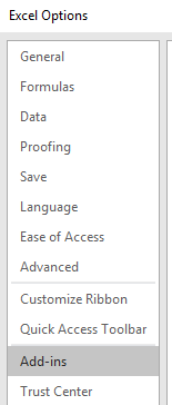
To do this, you have to get to the Excel Options. This will vary depending on which version of Excel you have, but in newer versions, you go to the File tab and select the Options button at the bottom of the page. Once there, you’ll want to select the Add-ins option.

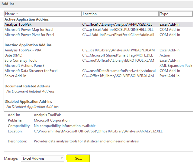
From there, you’ll have a list of all the Add-ins available. Then, next to the Manage button at the bottom, click on the Go button (highlighted in yellow).

After clicking the button, you’ll have a list of all the Add-ins that you can install.

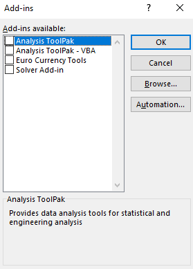
Click on the checkbox next to the Analysis Toolpak and then click OK.

Step 2: Running the Correlation Add-in

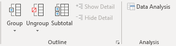
Now, if you go onto the Data tab, you should see off to the right, a button for Data Analysis, next to the Outline group.

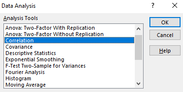
Clicking on the Data Analysis button will give you a lot of different options, but for this example, we’re just going to use the Correlation option.

Step 3: Selecting the Ranges to Evaluate

Next, you’ll be asked to select your Input Range. This is where you’ll enter the ranges that you want to compare. You can select either rows or columns. In most cases, you’ll probably leave the default, which is columns. You’ll want to select the columns you want to compare and specify if the label is in the first row.

Once you’ve selected your data along with where you want to output the data (I usually leave the default, which is New Worksheet Ply), then click on OK.

If you don’t have numbers in all your columns, you might see the following error come up:

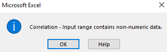
To fix this, you’ll need to look for any blank cells that might be in your data. If you have any if formulas that have a result of “”, then those will cause a problem as well. Either way, your data will need to be cleaned up to ensure that only numbers are in the range that you want to calculate correlations on.

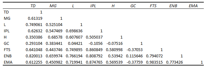
Once you’ve cleaned it up, depending on how many columns you selected, you should end up with something that looks like this:

Step 4 (Optional): Apply Conditional Formatting to the Correlation Matrix

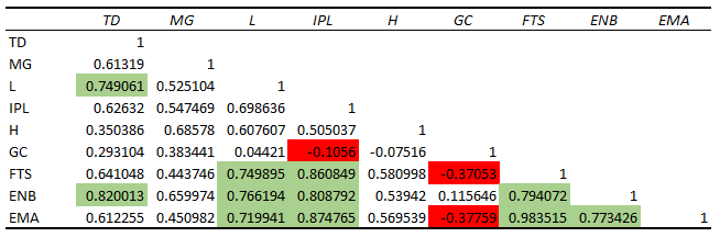
Although the matrix is technically complete, this is not an easy way to identify significant correlations, especially if you’re looking at several columns. This is where conditional formatting can help us.

What I’ll do is setup formatting so that anything between 0.7 and 0.99 shows up as green, and anything that is between -.1 and -.99 will be red to indicate a negative correlation. Now the matrix looks a bit easier to read since I can focus on areas of high or negative correlations:

For a detailed look at how to do conditional formatting, refer to this post.

Recreate a Correlation Matrix Using a Formula

That’s how you can create a correlation matrix in Excel, but what if you just want to look at the correlation between two pairs of data sets? In that case, you can use the CORREL function.

Back to my data set, I can use the CORREL function and select two data sets.

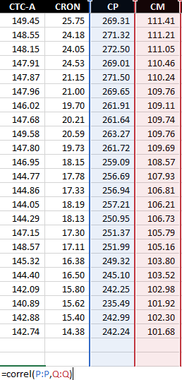
After hitting enter, it tells me the correlation of the two columns is 0.61. The one limitation of this is that you can only compare two data sets at a time. However, you don’t have to go through data analysis feature and can use this to put the correlation results in any way that you want.