H2Estockcorrelations

How to Calculate Correlations Between Stocks

Correlations can be helpful in determining if there is a pattern or relationship between two sets of data. It can be useful when looking at stocks as those that are highly correlated may move together in the same direction (note: this doesn’t mean their returns will be the same). And if you want to diversify, that’s not what you’ll want to accomplish. Instead, negatively correlated investments or ones that aren’t correlated at all may be more preferable in that situation. Below, I’ll show you how you can easily calculate correlations between multiple stocks from data that you can download from a source like Yahoo Finance.

Downloading the data

The first thing that’s needed when running correlations is to download at least two sets of data. In this example, I’ll download data for five stocks: Pfizer, Procter & Gamble, Tesla, Exxon Mobil, and Alphabet. None of those stocks is terribly similar to one another so there should be some decent diversification there.

Below, I’ve downloaded all the closing prices from Yahoo Finance for all of 2021. Here’s what that data looks like:
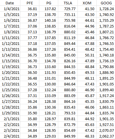
Stock prices download from Yahoo finance for five stocks.

The key is you want to make sure that the data is the same; you don’t want to have one stock showing a price at a different date than the other. They all need the same baseline. And that’s what the date field serves to do here. It itself isn’t necessary for the correlation calculation, but it’s just there to ensure that when you’re downloading and matching up data, everything lines up correctly to the right date.

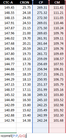
The CORREL() funciton is useful for doing just a quick correlation calculation

Using Excel’s CORREL function, you can quickly calculate the correlation between two stocks. Pfizer is in column B and Procter & Gamble is in column C. If I wanted to quickly calculate their price correlation, my formula would be as follows:

=CORREL(B:B,C:C)

It doesn’t matter which order the data is in but there are only two ranges that are used as arguments in this function. This formula tells me there is a 94% correlation between these two stocks, at least, over the past year. That’s incredibly high and it could be because these are two fairly safe, value-oriented investments. Now, I could repeat this process for the other stocks here but there’s a quicker way to do that.

Using the Data Analysis option

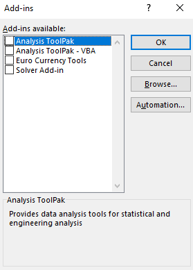
Excel has some built-in Add-ins that you can enable that can quickly do tasks like this for you. You can access the Excel Add-ins from the Developer tab or by going through File->Options->Add-ins->Excel Add-ins. Either approach will get you to the same place. And once you’re there, you just need to check off the option for the Analysis Toolpak:

Selecting the Analysis ToolPak Add-in.

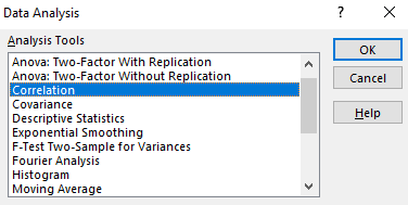
Once enabled, you will see the Data Analysis option on the Data tab. Clicking on that will give you many different options, including to do a Correlation:
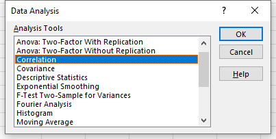
Selecting correlation from the Data Analysis options.

On the next screen, I’ll have the option to select an Input Range. Here, I can select more than just two columns:
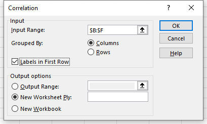
Correlation option in data analysis.

After clicking OK, Excel generates the correlation matrix for me in a new tab, saving me the time of doing all the calculations myself:

Correlation matrix for various stocks.

The lowest correlation noted here is between Tesla and Exxon Mobil, while the highest is between Pfizer and Procter & Gamble.


If you liked this post on How to Calculate Correlations Between Stocks, please give this site a like on Facebook and also be sure to check out some of the many templates that we have available for download. You can also follow us on Twitter and YouTube.

presentation-1454403_640

How to Make a Correlation Matrix in Excel

To find correlations between data points is useful when you’re trying to find a pattern or any sort of relationship. Below, I’ll show you how you can quickly do a correlation matrix as well as how to do a calculation if you’re only looking at two data sets to compare.

Step 1: Enabling the Data Analysis Add-on

One of the biggest challenges in creating a correlation matrix is just finding where the option to calculate the correlations is. In order to access it, you need to first enable the Data Analysis add-on.

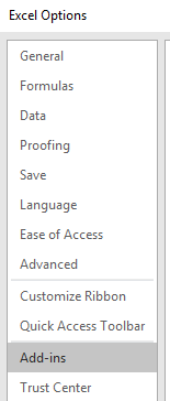
To do this, you have to get to the Excel Options. This will vary depending on which version of Excel you have, but in newer versions, you go to the File tab and select the Options button at the bottom of the page. Once there, you’ll want to select the Add-ins option.

excel options

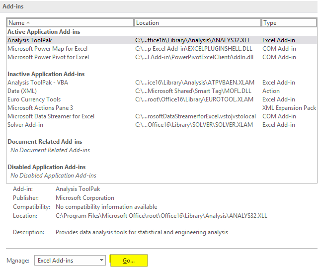
From there, you’ll have a list of all the Add-ins available. Then, next to the Manage button at the bottom, click on the Go button (highlighted in yellow).

excel add-ins

After clicking the button, you’ll have a list of all the Add-ins that you can install.

excel add-ins data analysis

Click on the checkbox next to the Analysis Toolpak and then click OK.

Step 2: Running the Correlation Add-in

Now, if you go onto the Data tab, you should see off to the right, a button for Data Analysis, next to the Outline group.

data analysis group

Clicking on the Data Analysis button will give you a lot of different options, but for this example, we’re just going to use the Correlation option.

data analysis correlation

Step 3: Selecting the Ranges to Evaluate

Next, you’ll be asked to select your Input Range. This is where you’ll enter the ranges that you want to compare. You can select either rows or columns. In most cases, you’ll probably leave the default, which is columns. You’ll want to select the columns you want to compare and specify if the label is in the first row.

Once you’ve selected your data along with where you want to output the data (I usually leave the default, which is New Worksheet Ply), then click on OK.

If you don’t have numbers in all your columns, you might see the following error come up:

correlation error

To fix this, you’ll need to look for any blank cells that might be in your data. If you have any if formulas that have a result of “”, then those will cause a problem as well. Either way, your data will need to be cleaned up to ensure that only numbers are in the range that you want to calculate correlations on.

Once you’ve cleaned it up, depending on how many columns you selected, you should end up with something that looks like this:

correlation matrix excel

Step 4 (Optional): Apply Conditional Formatting to the Correlation Matrix

Although the matrix is technically complete, this is not an easy way to identify significant correlations, especially if you’re looking at several columns. This is where conditional formatting can help us.

What I’ll do is setup formatting so that anything between 0.7 and 0.99 shows up as green, and anything that is between -.1 and -.99 will be red to indicate a negative correlation. Now the matrix looks a bit easier to read since I can focus on areas of high or negative correlations:

correlation matrix conditional formatting excel

For a detailed look at how to do conditional formatting, refer to this post.

Recreate a Correlation Matrix Using a Formula

That’s how you can create a correlation matrix in Excel, but what if you just want to look at the correlation between two pairs of data sets? In that case, you can use the CORREL function.

Back to my data set, I can use the CORREL function and select two data sets.

correl function

After hitting enter, it tells me the correlation of the two columns is 0.61. The one limitation of this is that you can only compare two data sets at a time. However, you don’t have to go through data analysis feature and can use this to put the correlation results in any way that you want.