How to Make a Map Chart in Excel

If you’re creating a dashboard or just want to visualize your data by what part of the world it’s coming from, a map chart can be a great way to accomplish that. Below, I’ll show how you can use a map chart to show data points at regional and global levels. And while you technically can’t use them with pivot tables, I’ll show you how you can use slicers to seamlessly drill down and dynamically update your chart.

Creating a global map chart

It should be easy to tell if the map chart is available on your version of Excel as the Maps icon stands out in the chart section:

If you see the maps option, then you have a compatible version to work with.

To set up the data to work with the maps chart all you need is a simple table that shows a location along with a value. In this example, I’ll focus on different country data. My data set shows the GDP per capita (in U.S. dollars) by country, courtesy of the World Bank. Here’s what a glimpse of what it looks like:

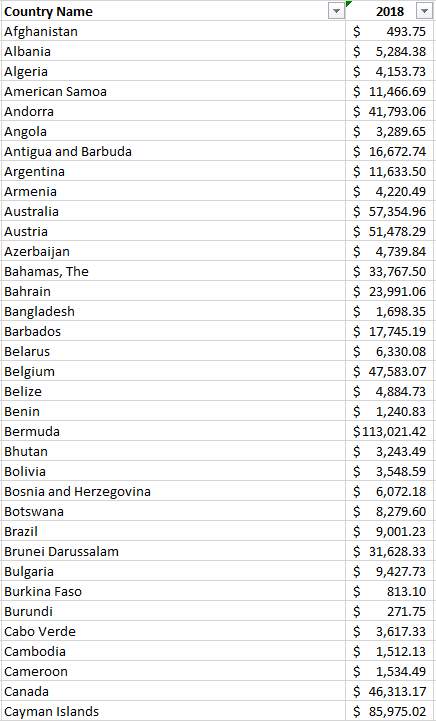
This table doesn’t look terribly great in text and it’s an ideal thing to visualize on a map. As long as your data looks like this and the country names are correct, you can just select this data set and go to insert the map chart, and you’ll get something that looks like this:

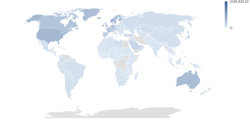
As you can see, the dark blue parts of the world have the highest GDP per capita while the lowest shades are on the bottom end of that scale. And the areas in grey do not contain data.

The map automatically adjusts based on how many countries you have included in your data set. If I only include data for Canada, the U.S., and Mexico, my map looks like this:

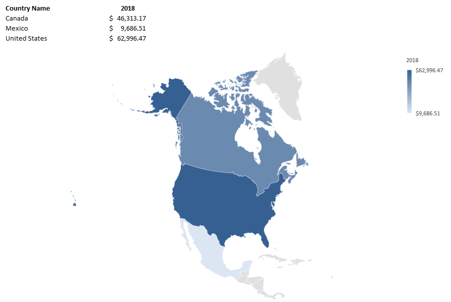
One of the cool things is you can really zero in on specific regions depending on your data set.

The one thing you might be disappointed to learn is that this type of chart does not work with pivot tables. But in the next section, I’ll show you how you can still drill down on the data and the chart using slicers.

Using slicers to break down the data

Using data from the Bureau of Economic Analysis, I downloaded data for per capita income by county in the U.S., below is what the table looks like:

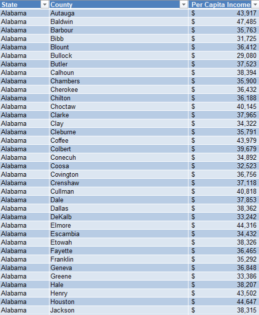
I had to do a bit of cleaning up the data to ensure that every line contained the state. And it’s also important to convert this into a table so that slicers will work with it.

With the maps chart, one of the things you’ll notice is you need to provide enough of a trail for Excel to be able to determine which location you are referring to. Cities, for example, could have the same names in multiple states or countries. And that’s why whether you’re looking at counties or cities, the more information you provide Excel, the more likely the chart will come out as you want it to.

When you first create a map chart it may not look as you expect it to as it could get the categories all wrong, especially if you have multiple fields. You’ll want to make sure that your series and categories are correctly set up if something looks off.

Under the Series, you should only have your values, such as in my example where it only contains per capita income:

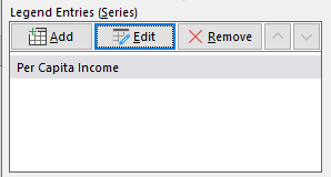
If there’s anything else in there, you may need to delete it and adjust your range. And for your values to show up as a scale (which I’d recommend, otherwise you’ll see a big legend with many colors), you’ll want to edit the legend and make sure the following option is selected:

You may also need to adjust the Horizontal Axis to ensure it includes all of your category columns. Again, this is if your map doesn’t look correct and the regions aren’t showing up correctly. Here is how my horizontal category axis looks like, showing both state and county:

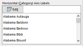
If it’s all set up correctly, your map chart should look something like this:

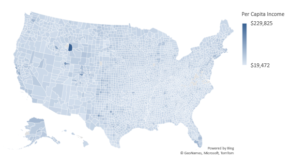
Now, because this is county-level data, it’s not easy to conceptualize what you’re looking at. But with the help of slicers, you can easily jump to different states. Since the data is in a table, you can add a slicer for the state. If you’re not familiar with how slicers work, check out this post. Although that’s for pivot tables, they’ll work the same within a table.

Once the slicers are in place, you can easily jump through and toggle between the different states. Doing so will automatically adjust your map chart which will now focus in on that specific state, just like when it narrowed in on North America when I only had data for three countries:

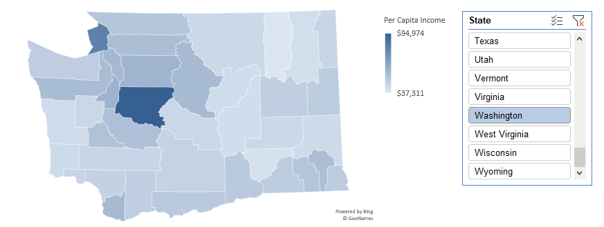
Just like with any other chart, you can hover over and see what the values are and the name of the county.

If you liked this post on how to make a map chart in Excel please give this site a like on Facebook and also be sure to check out some of the many templates that we have available for download. You can also follow us on Twitter and YouTube.