How to Calculate Stock Returns

In this post, I’ll show you how you can calculate stock returns using Google Sheets. However, you can use a similar approach in Excel by using the STOCKHISTORYFUNCTION.

First thing’s first — let’s pull in the historical data

For this example, I’m going to pull in the S&P 500’s historical values to see how the index has performed both in the past 12 months and over the course of several years.

To do that in Google Sheets, I’m going to use the GOOGLEFINANCE function which allows me to pull in historical prices. To get the values from the S&P 500, the ticker symbol I’m going to use is ‘.INX’ and to get the last year of data, I’m going to set my start date equal to TODAY()-365 and my end date will be TODAY(). Here’s the full formula:

=GOOGLEFINANCE(“.INX”,”price”,today()-365,today())

If you want to go back years, you can go as far back as 1970. For that, it’s easier to just manually enter that using the DATE function:

=GOOGLEFINANCE(“.INX”,”price”,date(1970,1,1),today())

If you don’t want to return 13,000 rows, you can add an argument at the end to set it to ‘Weekly’ prices (the default is daily):

=GOOGLEFINANCE(“.INX”,”price”,date(1970,1,1),today(),”weekly”)

Looking up the correct values

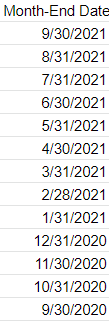
Once you’ve got the data loaded, then what you’ll want to do is enter the dates that you need values for. In this example, I’m going to use the last day of every month. For this, I can use the EOMONTH function. It takes two arguments: the start_date and the number of months. If I want the current month-end date, then I just set the second argument (months) to zero. As for start date, that can just be any date that falls within the month, which I can enclose within a DATE function. Here’s how the formula would look if I want the last day of September 2021:

=EOMONTH(date(2021,9,1),0)

But since I need to adjust this so that I can copy the formula down and have it automatically adjust, I am going to use the ROW function, which will return the current row number. Since I want the values to be increasingly negative as I copy down the formula (e.g. the current month should be 0, the following one -1, then -2, and so on), I will multiply this by a factor of negative 1 and add 1 to the total (to ensure the first value start at zero):

ROW(A1)*-1+1

That replaces the zero value from the earlier formula:

=EOMONTH(date(2021,9,1),ROW(A1)*-1+1)

And now, I can easily copy this formula down and my month-end dates will populate without requiring me to make any manual adjustments along the way:

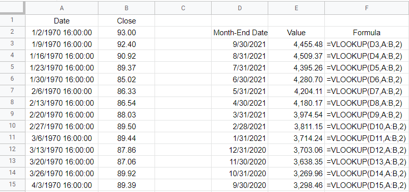
Next, I’ll do a lookup to get the values. And that’s as simple as a VLOOKUP on my dates, which are in column A with the corresponding values in column B. If you use weekly dates, then be careful not to set the last argument in the VLOOKUP function to false because you’ll end up with errors as the weekly values won’t always fall neatly on the end of the month. Instead, leave the last argument blank or set it to TRUE so that it finds the closest match. Here’s what that looks like:

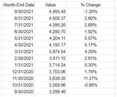
All that’s left at this point is to now just calculate the change in value. I can take the new value, divide it by the previous period’s value, and subtract one from it. This will give me a percent change:

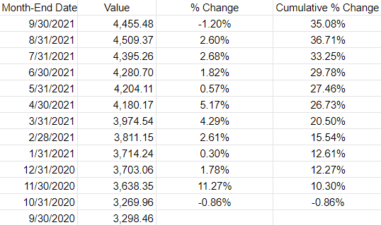
If I wanted to determine the cumulative % change since my first month-end date, then the old value would always remain the same — it would be the first date in the series. By freezing that cell, I can calculate the cumulative % change:

If you wanted to pull in the returns by year, you can do the same thing. All that changes is that instead of pulling in the month-end dates you will use the year-end dates. The main difference here is in calculating the different dates. Rather than multiplying by a factor of -1, you’ll need to use -12. And the starting date should be Dec. 1. Here’s how my formula looks like:

=EOMONTH(date(2020,12,1),ROW(A1)*-12+12)

And when I copy that down, it will automatically adjust for each previous year:

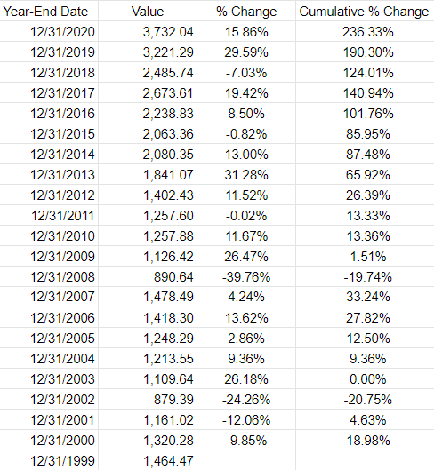
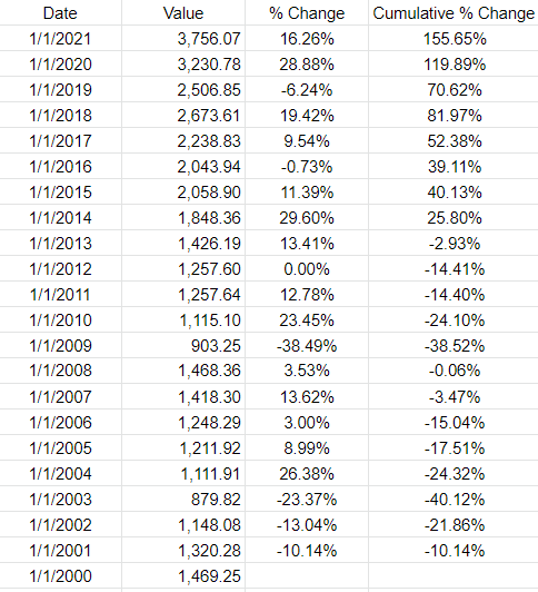
The one thing you may notice in Google Sheets is that the GOOGLEFINANCE function returns a timestamp for the date. Each day ends at 16:00:00. This can create some unintended results. For example, using the VLOOKUP function, if I use the date 12/31/2020, because it looks for an approximate match, it will actually return the value from 12/30/2020. Unless you add the timestamp, an exact match won’t work. And since a date with no time will by default by 0:00, the lookup of 12/31/2020 16:00:00 won’t be a match. One way to get around this is just to use a different date. Rather than using the EMONTH function, I can just adjust the date by reducing the year by 1. This is the formula I can use if instead I want to get the first day of the year:

=DATE(2021-ROW(A1)+1,1,1)

Using the ROW function again can allow me to automatically adjust the year. Here is the updated table:

If you liked this post on Using Tags in Excel, please give this site a like on Facebook and also be sure to check out some of the many templates that we have available for download. You can also follow us on Twitter and YouTube.