In this post, I’m going to show you how to group dates in a pivot table by month. By doing this, you can do analysis by month rather than individual day. And that will also make it easier to plot the data on a chart.
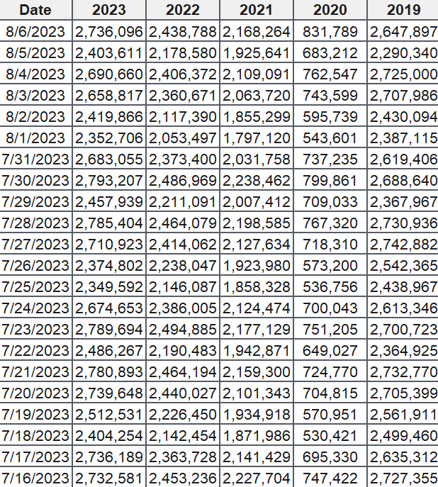
For this example, I’m going to use TSA passenger volumes as my data set and analyze them by month and year. Here is the data I’m going to use, which runs up until Aug. 6, 2023:
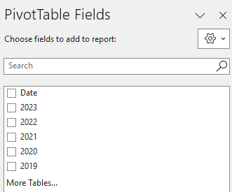
If I load this into a pivot table, my fields are as follows:
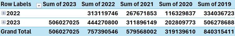
I have the date field which shows the current year’s dates. And there is also a field for each year, which contains the passenger volumes. If I put the Date in the Rows section of the pivot table and then years into the values section, then my pivot table looks like this:
There are a few things that I need to fix for this analysis to work:
I need to change each year field so that it is taking an average instead of summing the values. If I leave it as is, summing the values may not be helpful as the months are not going to be identical eah year. Taking an average will help smooth the data.
The formatting should be changed so that the values are separated by commas. This will make it easier to visually see the data. The numbers are too big and can be difficult to interpret in their current format.
The Row labels are broken down by year. But I already have the year values going across. This is not necessary and I need to have only the month values.
Here’s how to address these items.
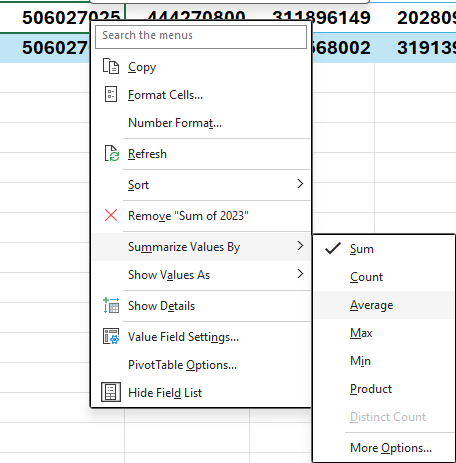
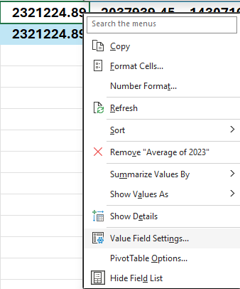
To change the year field so that it takes an average, right-click on the field and select the option to summarize as an average:
Repeat this for each field, so that everything says average. To fix the number formatting, right-click on each field and select Value Field Settings:
Change the formatting to Number and check off the option for the 1000 separator. Repeat these steps for the other fields as well.
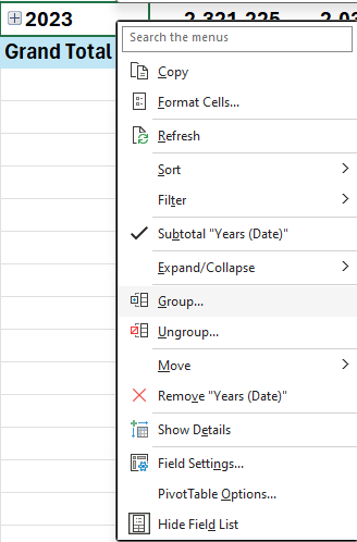
Next, for the date grouping, right-click on any of the date values and select the Group button:
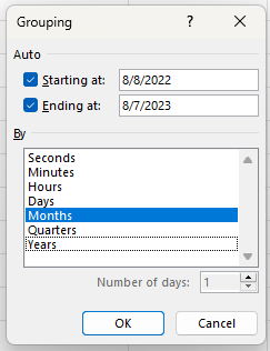
At the following dialog box, uncheck years and quarters and just leave Months:
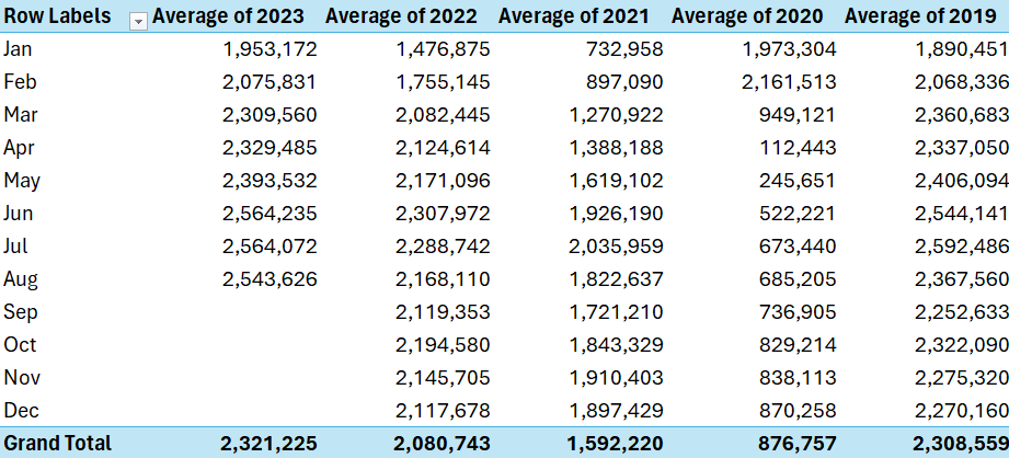
After making all those changes, my pivot table now looks like this:
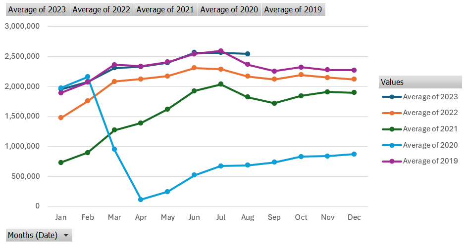
It’s now easier to compare the different months and years. And it’s also easier to put it on a chart. If I insert a line chart, it’s easy to spot the trends by a monthly and yearly basis:
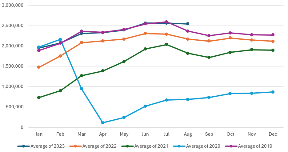
This is a PivotChart, as it evident from the grey drop-down options. If you prefer to get rid of the filters, go to the PivotChart Analyze tab and uncheck the Field Buttons option. Now you’ll have a cleaner chart layout. In the below example, I have also moved the legend to the bottom:
As you can see, by grouping your pivot table dates by month, it becomes easier to analyze data. And by not doing a daily analysis, it’s possible to look at the data from a year-to-date view to compare the monthly averages. This way, you are able to still see the story behind the data without having a crowded chart.
If you liked this post on How to Group Dates by Month in a Pivot Table, please give this site a like on Facebook and also be sure to check out some of the many templates that we have available for download. You can also follow me on Twitter and YouTube. Also, please consider buying me a coffee if you find my website helpful and would like to support it.
A histogram is a type of chart used to visualize the frequency distribution of a dataset. It represents how often different values occur within specific intervals or “bins” in a dataset. Histograms are particularly useful when you want to understand the distribution of continuous or discrete data and identify patterns, trends, or outliers in the data. They provide a clear and concise way to see the shape of the data and assess its central tendency and spread.
What the uses for a histogram?
Frequency Distribution
Histograms help you understand how data is distributed across different ranges or bins, revealing patterns or clusters in the data.
Identifying Outliers
With histograms, you can easily spot extreme values, or outliers, that may skew the chart.
Data Exploration
Histograms are great for data exploration and initial analysis, providing insights that may guide further investigation.
Data Comparison
You can compare multiple datasets or subsets of data to understand differences in their distributions.
How do you define bins for histograms?
One of the most important questions to ask yourself when creating histograms is how the bins should be defined and how big they should be.
Creating bins for histograms involves grouping the data points into intervals or ranges so that you can analyze the frequency distribution of the data effectively. The choice of the number of bins and their width can significantly impact the insights you gain from the histogram. There are various methods to determine the number and width of bins, and some common approaches include:
Square Root Rule
The square root rule suggests that the number of bins should be approximately the square root of the total number of data points. This method provides a simple way to determine the initial number of bins.
Sturges’ Formula
Sturges’ formula is a commonly used method to calculate the number of bins. It suggests that the number of bins (k) can be calculated as follows: k = 1 + log(n) where “n” is the number of data points. Sturges’ formula automatically adjusts the number of bins based on the data size.
Scott’s Normal Reference Rule
Scott’s rule considers the data distribution’s variability and suggests bin width based on the sample standard deviation (σ) and the number of data points (n): bin width = 3.5 * σ / (n^(1/3))
A larger standard deviation or more data points will result in wider bins.
Freedman-Diaconis’ Rule
This method takes into account the data distribution’s interquartile range (IQR) and the number of data points (n) to calculate the bin width.
Bin width = 2 * IQR / (n^(1/3))
The interquartile range is the difference between the 75th and 25th percentiles of the data.
Manual Selection
Depending on your domain knowledge and the specific insights you are seeking, you can manually choose the number of bins and their width. Adjusting the number of bins can highlight different aspects of the data distribution. With Excel, you can also do trial and error to see how many bins may be the best option for your chart.
When determining the bins, you should consider the following points:
Avoid too few bins, as this may oversimplify the data distribution and hide important details.
Avoid too many bins, as it may result in overfitting and obscure the underlying patterns.
Consider the data range and the resolution you want to achieve in the histogram.
Once you have determined the number of bins or their width, you can create the bins in Excel by manually specifying the bin ranges in a new column or using Excel’s built-in histogram function, which will automatically calculate the bins for you based on the data.
Creating a histogram chart in Excel
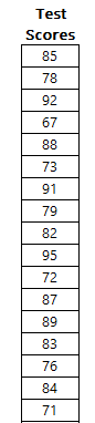
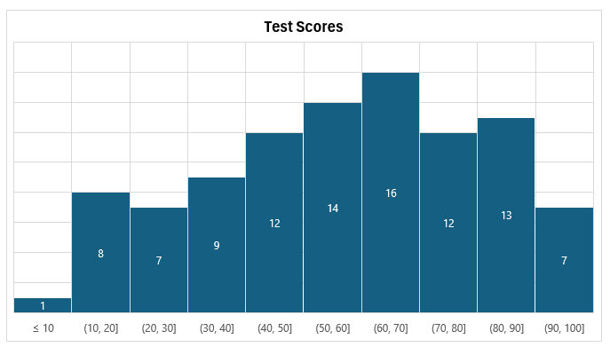
In creating a histogram in Excel, I’m going to use test scores on an exam as an example. This is an excerpt of my data set:
Here are the step-by-step instructions to creating a histogram chart in Excel.
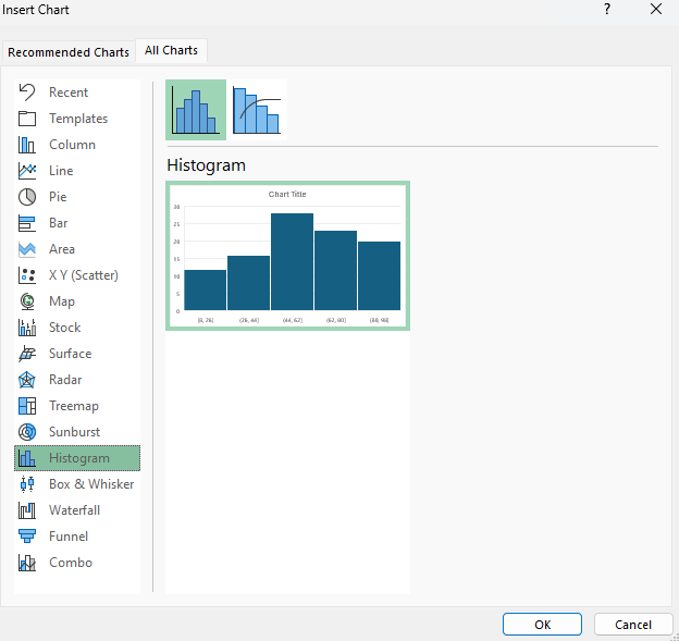
Step 1. Select the histogram chart
Excel makes it easy to create a histogram. All you need to do is select the entire data set and then click on the option to insert a chart from the histogram section:
As you can see from the preview, Excel has already set up some bins based on the data, so you may not even need to worry about setting them up yourself.
Step 2: Modifying your bins (if necessary)
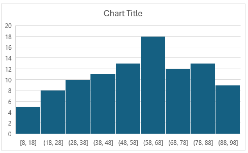
This is the chart that Excel has created for me based my data set:
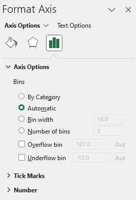
It has created bins of equal size based on the data set. However, you may not agree with the cutoffs given they are a bit random (e.g. 8-26, 26-44, etc.). To change this, you can right-click on the x-axis and select the option to Format Axis. From there, there is a section for the different bin options:
The default options is set to automatic. However, in this situation you may want to consider using either a set bin width or changing the number of bins. As you can see from the greyed out numbers, Excel has created 5 bins with a width of 18 each. If you change the bin width to 10, then Excel starts from the lowest value of 8 and adds 10, and continues on:
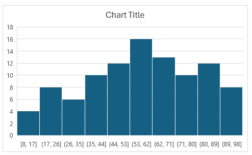
This has created 9 bins. But suppose you want 10 bins. You can change the number of bins to 10 manually. And when doing so, this is the chart Excel creates:
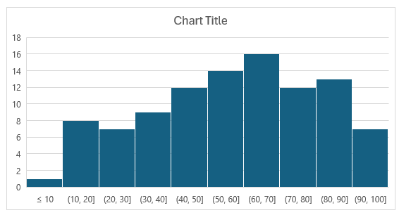
Now the bin width is set to 9. For test scores, this still may not be ideal, as the cutoffs don’t make logical sense. Ideally, they would be in increments of 10 and be round bin numbers. To fix this, what you can do is to set a bin width of 10. And then, set the underflow bin to 10. This means that anything less than or equal to 10 will fall into the first bin. This becomes a catch all for any values of 10 and under, even if the data starts at 8. Now, the histogram looks like this:
This is a much cleaner look with cutoffs that make more sense. One thing to note is that while there does appear to be an overlap in the bins, that’s not the case. For the (10,20] bin, it counts the number of values that are greaterthan 10 up to and equal to 20. For the (20,30] bin, it counts values greater than 20 that are up to and including 30.
Step 3: Apply formatting (optional)
Once you’re satisfied with the number of bins and their width, the last step is to change the formatting, assuming you want to change the look of it. This can involve changing the histogram’s colors, adding or removing gridlines, adding data labels, as well as any other changes you might normally make to a chart.
In my example, I’ve modified the title, added vertical gridlines, and added data labels to show the frequency count, and also removed the axis to the left:
If you liked this post on How to Make a Histogram Chart in Excel, please give this site a like on Facebook and also be sure to check out some of the many templates that we have available for download. You can also follow me on Twitter and YouTube. Also, please consider buying me a coffee if you find my website helpful and would like to support it.
The TREND function in Excel is a powerful tool that allows users to perform linear regression analysis and make predictions based on existing data. This function is particularly valuable for professionals dealing with data analysis, financial modeling, and forecasting. In this article, I will go over how the function works, and provide step-by-step instructions on how to utilize it in your Excel worksheets.
Using the TREND function
To use the TREND function, follow the steps below:
1. Organize the data
Before you can use the function, you need to have your data organized so that it includes at least two columns. One needs to be for the independent variables, or the x-values, and another one for the dependent variables, or y-values. It is necessary for the data to be aligned correctly so that the information correctly relates to one another (i.e. you don’t want the wrong values lined up next to one another).
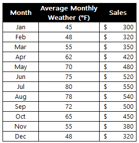
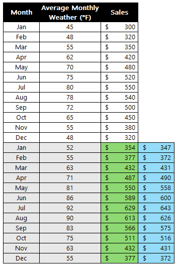
Below is sample data for a company which sells seasonal products. In warmer weather, revenue rises while in cooler temperatures, sales are lower.
2. Calculate the Trend Line
With the data populated, you can now enter it into the TREND function in Excel. This involves specifying the following arguments:
known_y’s
known_x’s
new_x’s
constant
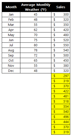
In the above example, the known_y’s are the sales, the known_x’s are the average monthly temperatures. If I don’t fill in any new_x’s or specify the constant, the function will still try and plot out the rest of the values:
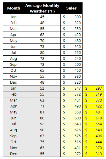
The problem in this scenario is that it doesn’t take into account the temperature; it simply assumes a similar trend as before. The function is much more useful if I have forecasted monthly temperatures. That way, the trend calculation will take that into account. Suppose I fill in the data, telling Excel that I expect the temperatures to be much warmer over the next 12 months:
With the previous forecast off to the right, you can see that the TREND function has adjusted to reflect the newer information. Thus, the more data you plug into the function, the more reliable the forecast will be. Otherwise, it will simply assume the same patterns will repeat from before, which may not necessarily be the case.
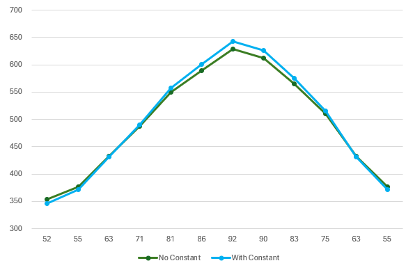
There is an additional argument in the function that you can also adjust, and that is the constant. If you set it to false it will be 0. If set to true, then the formula will calculate it. This is the b variable which is part of the y=mx+b equation. If you expect there to always be a minimum, a constant amount, then you may want this to be calculated. If, however, the data can fluctuate wildly, then you may want to set it to true so that there is no intercept. Here’s a comparison with the above data both when there is a constant and when there isn’t:
The forecast in green is where the argument is set to false (constant is set to zero) and blue is where it is true and a constant is calculated. From the chart below, you can see that there isn’t a big difference but the highs are higher and the lows are lower when there is a constant. This may, however, not always be the case as it will depend on your individual data set.
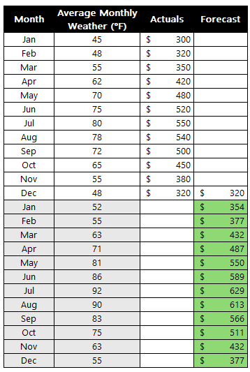
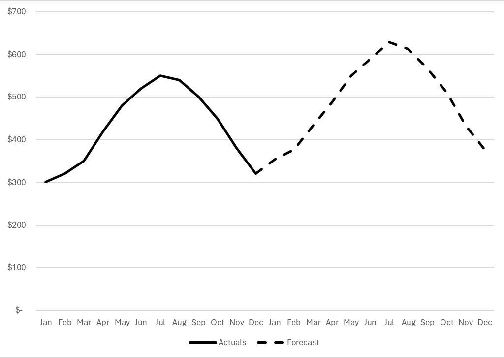
Create a chart to differentiate between actuals and forecast
One thing you may find helpful to do when creating a forecast is to put those amounts on a different column:
By doing this, you leave yourself space to add actuals later on and to compare them against your forecast. You can also create a chart with the forecast being a different series. In the below chart, I have used a dotted line to show the forecast while the actuals remain solid. For the first forecast amount, I set it to the same as the actual. This way, when I create the chart below, there are no gaps and it is merely a continuation of the line.
If you liked this post on How to Use the Trend Function in Excel, please give this site a like on Facebook and also be sure to check out some of the many templates that we have available for download. You can also follow me on Twitter and YouTube. Also, please consider buying me a coffee if you find my website helpful and would like to support it.
A popular investing strategy is dollar-cost averaging. With dollar-cost averaging, people invest a fixed amount of money into an investment on a recurring basis, regardless of whether the price has gone up or down. In this post, I’ll go over how it works, the benefits and disadvantages of dollar-cost averaging, along with a step-by-step guide on how to do it in Excel, using the stock market as an example.
What is dollar-cost averaging?
Dollar-cost averaging is an investment technique that takes the emotional aspect out of investing by spreading purchases over regular intervals, typically on a monthly basis. This means that regardless of market conditions or how you feel about an investment, you invest the same fixed-dollar amount on a recurring basis. When a stock’s price is low, that means you can buy more shares since they are cheaper. And when the price is higher, you buy fewer shares. But the end result is that you’re investing the same amount of money each time.
Why investors might use dollar-cost averaging
Below are the main reasons investors may want to consider using dollar-cost averaging:
Risk Mitigation
Dollar-cost averaging reduces the impact of market volatility on investment returns. By investing consistently over time, investors avoid the risk of investing a lump sum at the market peak and potentially suffering significant losses if the market subsequently declines. If the stock goes up in value, then that means your earlier buy-ins are generating profits and you’re buying into the rally. If the stock is going down, then you’re buying more of it and are averaging down. The benefit here is that as long as the business and investment remains sound, there’s a good chance that the stock will recover from a drop. Buying low could end up setting you up for some great returns.
Disciplined Approach
By dollar-cost averaging, investors establish habits that can help them resist the temptation to make impulsive decisions based on short-term market conditions. The investor remains focused on the long term and that can help lead to more rational decisions.
Ease of Implementation
Dollar-cost averaging is simple to execute, whether you’re an experienced investor or a novice one. You don’t need to do any complex analysis and instead just need to do the same thing every month or every period you plan to buy stock. By making the process easy, it makes it easier to adhere to.
Benefits of dollar-cost averaging
There are several advantages to using dollar-cost averaging:
Emotional Discipline
Emotions can often drive investment decisions, leading to irrational actions such as panic selling during market downturns or chasing after hot stocks during bull markets. Dollar-cost averaging can ensure you aren’t being reactive or making emotional decisions, which can lead to losses and risky behavior.
Lower Average Cost
Provided that you’re investing in a quality business that will grow over time, dollar-cost averaging can keep your average cost down. That’s because you’re buying more shares when prices are low, and thus, are able to average down. And if the investment grows over time and its value increases, so do your profits. By making incremental purchases along the way, you don’t need to worry about buying at the peak.
Reduced Timing Risk
Timing the market is notoriously challenging, even for seasoned investors. Dollar-cost averaging mitigates timing risk by spreading investments over time, reducing the impact of market fluctuations on the overall portfolio. Since you’re buying stock at regular intervals, there’s no temptation to time the markets and you get a more balanced investing strategy.
Flexibility and Scalability
Dollar-cost averaging makes it easy for anyone to build up their position in a stock. Whether you can afford to invest $5,000 or $500, you can spread the amount you plan to invest over the course of a full year into 12 monthly payments. Brokerages nowadays offer low or no-cost commissions, making it easy to justify investing even a modest amount; there’s no need to make a big buy-in.
Disadvantages of Dollar-Cost Averaging
These are the biggest drawbacks of using dollar-cost averaging:
Potential Missed Opportunities
The biggest downside of dollar-cost averaging is that if the price of a stock has dropped significantly, you are not investing more than your recurring amount. Even if the stock becomes a steal of a deal, with dollar-cost averaging you could potentially miss out on that opportunity since you aren’t making a big purchase at the time a stock becomes oversold or is trading at a big discount.
Increased Transaction Costs
In the event you aren’t using a low-cost brokerage and where you are incurring transaction fees, you could be incurring high expenses relative to your investment amount. This can be particularly troublesome when you’re making small investment amounts and fees will end up representing a big chunk of your overall investment. In these situations you may either want to increase your recurring investment amount, or simply not deploy dollar-cost averaging.
Diversification Limitations
Dollar-cost averaging is more effective when investing in a few stocks. It wouldn’t be practical or efficient if every month you had to invest the same amount in 10 or more different stocks. It can quickly become a time-consuming process, one that might not be worth sticking to. That’s why when investors talk of dollar-cost averaging, it usually relates to a small number of stocks, or perhaps even just one.
Market Trend Irrelevance
Dollar-cost averaging may not provide good returns in a bear market. When the market keeps going down, buying more simply ends up increasing your losses since you’re investing more during a downtrend. If you are going to use dollar-cost averaging, you need to have confidence in the business you’re investing in and be willing to be patient enough to hang on in the event of a bear market. If you need to sell your investment within a few weeks or months, dollar-cost averaging may not be a suitable strategy for you.
Step-by-Step Guide to Dollar-Cost Averaging
Here are the steps to take if you want to get started with dollar-cost averaging:
1. Set Investment Period
Determine the time interval for your investments. Monthly investments are common, but you can choose any frequency that suits your financial situation.
2. Allocate Investment Amount
Decide on the fixed amount you want to invest during each interval. This can be any amount that fits your budget and investment goals.
3. Choose Investment(s)
Select the asset or assets you want to invest in regularly. This can be individual stocks, exchange-traded funds (ETFs), mutual funds, or any other investment vehicle.
4. Start Investing
Begin investing the fixed amount at the chosen intervals, regardless of the asset’s price. Maintain consistency over the set investment period.
5. Monitor and Adjust
Regularly review your investment strategy and portfolio performance. Adjust the investment amount or asset allocation if your financial situation or investment goals change.
How to Calculate Dollar-Cost Averages in Excel
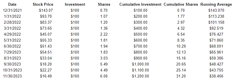
If you’ve begun dollar-cost averaging and want to know what the average cost of your investment is, you can do this easily in Excel. Create a table with the following headers: Date, Stock Price, Investment, Shares, Cumulative Investment, Cumulative Shares, and Running Average.
The Date relates to when the stock was purchased.
The Stock Price is what the stock price was when it was purchased.
The Investment is the total investment amount. This should be the same amount each period.
The Shares field is the number of shares purchased. This is the Investment total divided by the Stock Price.
The Cumulative Investment field is the sum of the Investment field up until the current date.
The Cumulative Shares field is the same thing, except it calculates the number of shares purchased up until the current date.
The Running Average takes the Cumulative Investment and divides it by the Cumulative Shares. Here’s an example of how dollar-cost averaging would have worked if you used to approach with Novavax, beginning in December 2021:
As you can see, with the very first row and very first purchase, the running average is the same as the stock price. But as the stock declines in value over the year, the running average becomes lower.
If you liked this post on How to Do Dollar Cost Averaging in Excel, please give this site a like on Facebook and also be sure to check out some of the many templates that we have available for download. You can also follow me on Twitter and YouTube. Also, please consider buying me a coffee if you find my website helpful and would like to support it.
Introducing the Ultimate Bank Reconciliation Excel Template – your time-saving companion for hassle-free financial management!
Are you tired of spending hours manually matching transactions and dealing with duplicates during your bank reconciliations? Look no further! This downloadable Excel file is here to revolutionize the way you handle your finances. Packed with powerful features and user-friendly functionalities, this template will streamline your reconciliation process like never before.
Automated Transaction Matching: Say goodbye to tedious manual matching. This Excel template is equipped with an intelligent algorithm that automatically matches transactions, making your reconciliation process a breeze. Experience unmatched efficiency as the template swiftly identifies and pairs up corresponding transactions, freeing up your valuable time.
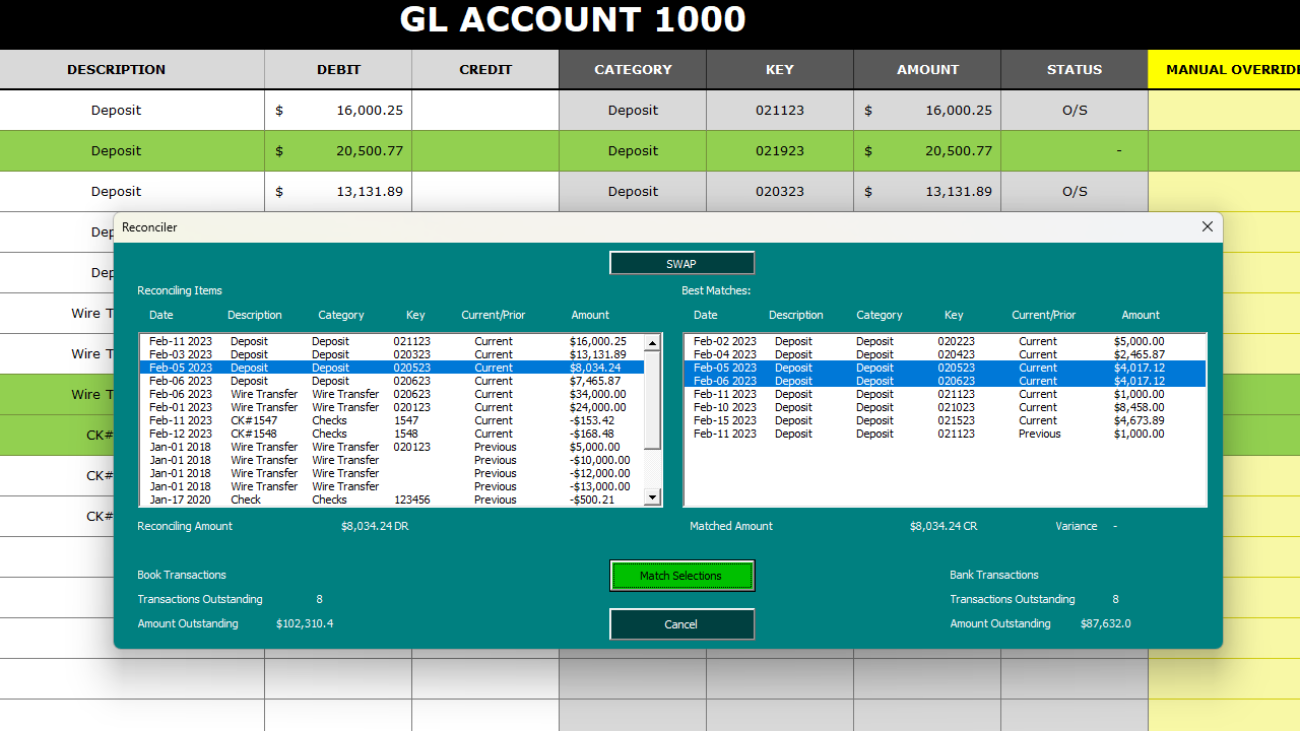
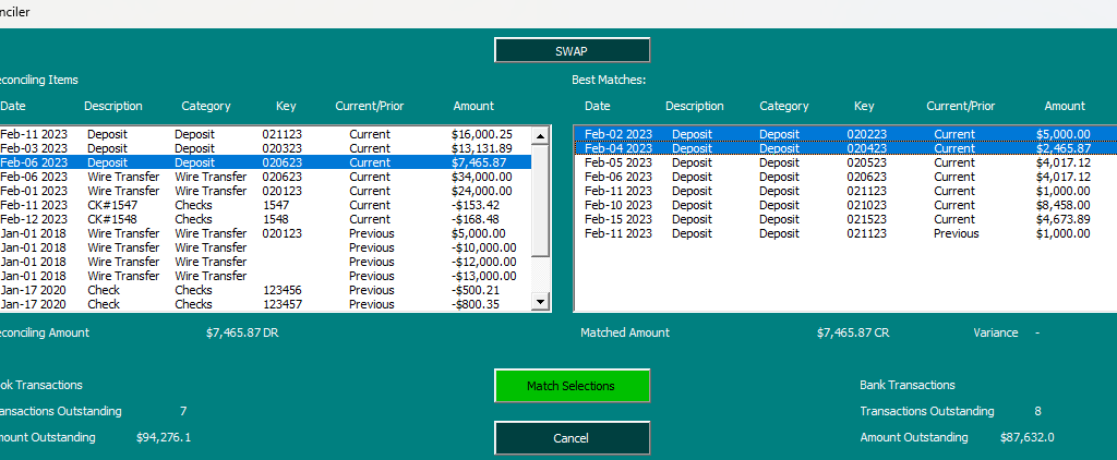
Effortless Manual Matching: Whatever the template doesn’t end up matching, you can do so manually using the Reconciler. It’s a much easier process than the manual approach as once you select a transaction, it will find related transactions that you can match the transaction to. Simply review the related items displayed, and with a few clicks, you’ll have your transactions matched accurately and swiftly.
Duplicate Detection: This template also checks for duplicates and will be careful not to match any items where there is a duplicate entry. You can still match these transactions manually using the Reconciler, but you won’t have to worry about the template automatically matching items where there are duplicates. This helps ensure accuracy and integrity when doing the automatic matching.
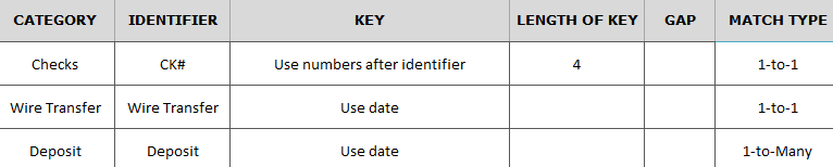
Flexible Matching Rules: Take full control of your reconciliation process with customizable matching rules. The Excel template empowers you to create rules to automatically match transactions on a 1-to-1 basis or 1-to-many, tailored to your unique needs.
By creating these rules, you can specify how a transaction should be classified.
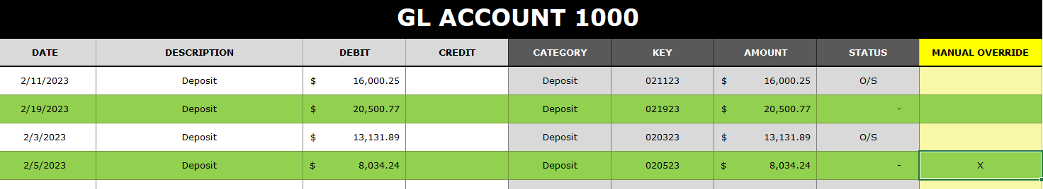
In the above example, if a description contains CK#, then it will belong to the ‘Checks’ category. For the key, which is used to help match a transaction, it will take the next 4 numbers. So if you have CK#1234, then 1234 would be the key. For a transaction to automatically match, it will need to be part of the same category, have the the same key, and amount. In the case of 1-to-1 matches, it will only need to find another transaction that matches this criteria. The one exception is if there is a duplicate; in that case, the transactions won’t automatically match. The auto-match is designed to minimize false matches.
For the Wire Transfer example above, it will simply use the date as the key. Since it’s a 1-to-1 match, it will look for another Wire Transfer on the same date with the same amount.
The deposit example shown above is slightly different in that it relies on the date but it is a 1-to-Many match type. However, this can also work as a many-to-many matching type as well. That’s because it will look for all of the deposits on that date, across the book, bank, and previous outstanding items. Only if the total of all the deposits on that date are a match will the auto-match rules kick in and say that everything is a match. You might use this type of matching if you have multiple deposits on the GL side that total just a single deposit amount on the bank side, or vice versa.
Easy Overrides. If you need to force a match, you can do so by entering any value in the ‘Manual Override’ column. This will clear the O/S status and indicates that the transaction has been matched. In the example below, just entering an ‘X’ is enough to mark off a transaction as being reconciled:
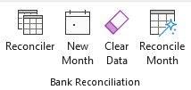
Quickly Generate Reports and Start a New Month: With just a click of a button, this Excel template generates a comprehensive report summarizing outstanding items. Gain valuable insights into your financial status and easily identify discrepancies that require attention. Stay on top of your bank reconciliations with accurate, up-to-date information at your fingertips. Clicking on the Reconcile Month button will summarize your outstanding items. You can also clear all the data with the Clear Data button. Click the New Month button when you’re done reconciling and want to close out the month. It will transfer all your current outstanding items to the previous outstanding items tab.
Try the bank reconciliation template for yourself!
Whether you’re a small business owner, a financial professional, or an individual managing personal finances, this Bank Reconciliation template is your go-to solution. Experience unparalleled ease, accuracy, and efficiency in your reconciliation process. Save time, reduce errors, and take control of your financial management like never before.
Best of all, you can try it out for free to see how you like it. Download the trial version here. If you decide you want to buy the full version without restrictions and full VBA code available, click on the following button:
If you like this Bank Reconciliation template, please give this site a like on Facebook and also be sure to check out some of the many templates that we have available for download. You can also follow me on Twitter and YouTube. Also, please consider buying me a coffee if you find my website helpful and would like to support it.
Combinations and permutations are fundamental deal with the arrangement and selection of objects or elements from a set. While both combinations and permutations involve counting possibilities, they differ in terms of the order and repetition of elements. In this post, I’ll show you how to calculate both permutations and combinations in Excel, both with and without replacement and repetition.
What is a permutation?
A permutation refers to an arrangement of objects from a set, where the order matters. In other words, permutations consider the different ways in which objects can be arranged. For example, let’s take the set {A, B, C}. The permutations of this set would be ABC, ACB, BAC, BCA, CAB, and CBA. The number of permutations can be calculated using the formula:
nPr = n! / (n – r)!
Where n represents the total number of objects in the set and r denotes the number of objects being selected for each arrangement. The exclamation mark denotes factorial, which means multiplying a number by all the positive integers less than it down to 1.
Suppose you want to consider all 26 letters of the alphabet — this would be the n value. Now, if you want to know all the different permutations when selecting 3 characters, that would be your r value. To calculate the number of different permutations, your formula would be as follows:
nPr = 26! / (26 – 3)!
This gets simplified to:
nPr = 26! / 23!
Rather than doing this complex calculation, you can first cancel out the numbers going up until 23 on each side. Then you’re left with the following:
26*25*24 = 15,600
This tells us that there are 15,600 different permutations when selecting the three letters from the alphabet. The preceding formula assumes that you are not replacing objects. If, however, you are replacing them then that means you can select the same item multiple times. In this situation, the formula for calculation permutations with replacement is as follows:
=n^r
When choosing 3 letters from the alphabet, the result would be:
26^3 = 17,576
In this situation, you have will have more possible permutations since the objects can repeat.
What is a combination?
If you’re talking about combinations, then the difference here is that you don’t consider the order as you would with permutations. In the earlier example where the set was {A,B,C} and you needed to select three characters, there would only be 1 combination. That’s because whether it’s ABC, BAC, CAB, or any other order of the characters, that’s irrelevant since combinations don’t care about order. The letters are all the same, and thus, there would only be 1 possible combination.
The number of combinations can be determined using the formula:
nCr = n! / (r!(n – r)!)
Let’s do this again, when selecting 3 letters from the alphabet:
nCr = 26! / (23! (26-23)!)
That formula simplifies to this:
nCr = 26! / 23! (3)!
And again, up until 23, everything gets canceled out, leaving the following:
nCr = (26*25*24)/(3*2*1)
This is the same as the result from the permutation calculation but the difference is that the denominator is now larger; it is calculated as the r factorial. Upon completing this formula, the result is:
15,600/6 = 2,600
This is the number of permutations divided by the factorial of 3, the number of selections. If there are replacements and you select the same item multiple times, this is the formula:
(n + r -1)! / (r!(n-1)!)
This results in the following calculation:
(26 + 3 -1)! / (3!(26-1)!)
This simplifies to:
(28)!/(3!(25)!)
Which further simplifies to:
(28*27*26)/(3*2*1) = 3,276
How to calculate permutations and combinations in Excel
In the above examples, I showed you how you can calculate permutations and calculations manually. But with Excel, there are formulas that can do the work for you.
To calculate permutations, we use the PERMUT function when there are no replacements. In the first example where there were 3 items chosen from a set of 26, this is the PERMUT formula:
=PERMUT(26,3) => 15,600
It returns the same result. If there are replacements, then the PERMUTATIONA formula is used:
=PERMUTATIONA(26,3) => 17,576
For combinations, the default function is COMBIN:
=COMBIN(26,3) => 2,600
And when there are replacements, COMBINA is used:
=COMBINA(26,3) => 3,276
These results all match up with the calculations from the previous examples, where they were done manually.
How to calculate the Powerball odds
For the Powerball, there are two draws that happen. The first is where 5 numbers are chosen from 69 possible items. Then, in the second draw, there is 1 number that selected from 26 possibilities. When dealing with probabilities, when we want both events to happen, we need to multiply the odds. The first step will be to calculate the individual combinations. Since there is no replacement, the formula for the first draw is as follows:
=COMBIN(69,5) => 11,238,513
For the second draw, the calculations straightforward since there is only 1 item selected from 26 possible options, so there can only be 26 combinations. Thus, to calculate the Powerball odds where you win both the first draw and the second draw, you need to multiple the odds of winning the first draw by the odds of winning the second draw:
=11,238,513 x 26 = 292,201,338
This tells us that the odds of winning both draws are 1 in 292 million.
If you liked this post on How to Calculate Combinations and Permutations in Excel, please give this site a like on Facebook and also be sure to check out some of the many templates that we have available for download. You can also follow me on Twitter and YouTube. Also, please consider buying me a coffee if you find my website helpful and would like to support it.
Microsoft Excel is a powerful spreadsheet software that people use for data analysis, calculations, and reporting. While Excel is primarily designed for managing and manipulating tabular data, many users have explored using it as a database. In this article, I will go over the pros and cons of using Excel as a database, highlighting its limitations and advantages compared to SQL and other alternatives.
Benefits of using Excel as a database
1. Familiarity and Accessibility
Excel enjoys widespread usage, and millions of users are already familiar with its interface and basic functionalities. It is easily accessible and requires no additional software or technical expertise to get started. This means no costly support bills as there are many users all over the world who can provide expertise on spreadsheets. And it’s already included in Microsoft 365, which many businesses already pay for.
2. Quick and Easy Data Entry
Excel provides a user-friendly environment for entering and editing data. Its intuitive grid layout allows for easy data input, and its familiar formula syntax enables simple calculations and data manipulation. You can also create templates for data entry so that it is customized to your company’s needs. Through userforms and visual basic, you can even create wizards that walk users through personalized data entry screens.
3. Simple Sorting and Filtering
Excel offers basic sorting and filtering capabilities that can be helpful for simple data analysis and organization. Users can sort and filter data based on specific criteria to extract relevant information quickly. This can make it easy to review and analyze data on-the-fly. Slicers also add convenience and can make filtering options even easier, giving users the ability to quickly apply filters with just a few clicks of a mouse.
4. Flexible Data Visualization
Excel provides various charting and graphing tools to visualize data effectively. Users can create professional-looking charts and graphs without the need for complex coding or external software. Pivot tables and pivot charts can be created within a few seconds and Excel has many chart templates available that can quickly summarize and display data. You can even create complex 3D bubble charts for more advanced models.
5. Low Learning Curve
Excel’s user-friendly interface and widespread familiarity make it more approachable for non-technical users. In addition to Microsoft’s tutorials, you can find help on message boards, and other websites, like this one, that can help you learn how to use Excel. There are also many YouTube videos covering tutorials as well. Oftentimes, you’ll find users with similar or even the exact problems you are experiencing, making it easy to find a solution with a simple search. In contrast, SQL and other database systems often require specialized knowledge and training.
6. Cost-Effectiveness
Excel is usually included in the Microsoft Office suite, which is commonly available in many organizations. Dedicated database systems may require additional licensing costs and infrastructure investments. With Excel, you just pay a recurring fee for Microsoft 365. And if you have an older off-the-shelf Excel product, you can use it indefinitely without having to pay a subscription fee.
7. Quick Prototyping and Ad Hoc Analysis
Excel’s ease of use allows for rapid prototyping and ad hoc analysis. Users can quickly create and modify data structures, perform calculations, and experiment with different scenarios without complex setup or formal data modeling.
Disadvantages of using Excel as a database
1. Limited Scalability
Excel is not designed to handle large datasets or complex data relationships. It has a practical limit on the number of rows (1,048,576 in Excel 2019) and can become sluggish when dealing with vast amounts of data. Additionally, as the file size grows, it can lead to performance issues and increased chances of data corruption.
2. Lack of Data Integrity and Security
Excel lacks built-in mechanisms for ensuring data integrity and enforcing strict security measures. It offers limited data validation features and minimal control over user access and permissions. This makes it prone to human errors, accidental data modifications, and unauthorized access. While macros, locked cells, and additional controls can be added to make a file more sure, they’re by no means ironclad; if you need to keep information confidential, then it’s best not to hold the data in Excel.
3. Lack of Concurrent Access and Collaboration
Excel files are typically stored on local machines, making it challenging for multiple users to collaborate simultaneously. Sharing and managing Excel files across different users can lead to version control issues and data inconsistencies. And if you’re using macros, then multiple users cannot be in the same file at once. This is one of the biggest drawbacks of trying to use Excel as a database and it’s one of the first questions I ask people who want to create a file that multiple people are using — do they need to be in it at the same time? If so, then Excel isn’t the right solution.
4. Limited Data Analysis and Reporting Capabilities
Excel’s analytical capabilities are limited compared to dedicated database systems like SQL. It lacks advanced querying capabilities, complex aggregations, and data mining functionalities, which can hinder advanced data analysis and reporting needs. While advanced users can create complex and custom reports, for those who aren’t comfortable doing it themselves, they may prefer using a different system.
Should you use Excel as a database?
Excel has lots of great functionality and by now it should be clear that you can use it as a database. However, the more important question is whether you should do so. There are three questions you can ask yourself to help make that decision:
Do multiple people need to be in the file at the same time?
Do you have a large database that may require more than 1 million rows in a single table?
Are you holding sensitive information (e.g. credit cards, social security numbers) in your database?
If you answer yes to any of those questions, then Excel probably isn’t going to work for you. But if you answered ‘no’ to all of them, then you may benefit from storing your data in Excel and using it as a database.
Regardless of what IT experts may tell you, there are situations where Excel can be used as a database and where it makes sense to do so, especially when the alternative is a costly system which requires ongoing maintenance and where support can be expensive.
If you liked this post on Whether You Can Use Excel as a Database, please give this site a like on Facebook and also be sure to check out some of the many templates that we have available for download. You can also follow me on Twitter and YouTube. Also, please consider buying me a coffee if you find my website helpful and would like to support it.
A column chart can be useful in data analysis to show growth, compare values, and display values by period. One of the drawbacks of a column chart is that as you add more data series and values to compare against, it starts to stretch out your chart. And when that happens, the data becomes more difficult to read. One way to conserve some space and to create a nice visual is by embedding one column chart within another. By doing this, you can show relative values. For example, one column chart might show total sales, while the embedded chart can show how much a particular product or geographical area accounted for.
Creating the column chart
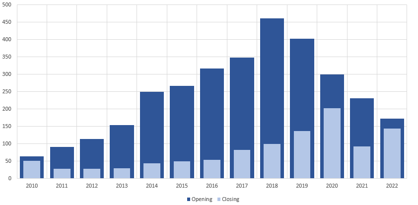
In this example, I’m going to use the data set from the following webpage, which shows brewpub openings and closings by year (https://www.brewersassociation.org/statistics-and-data/national-beer-stats/).
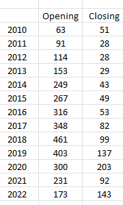
I’ve created a table of the data by year:
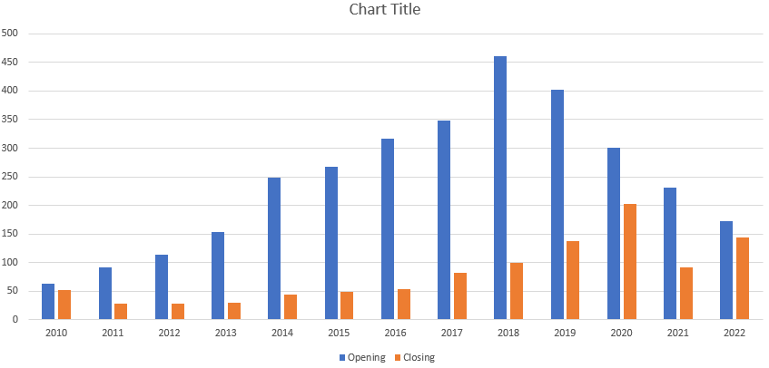
In this example, I’m going to use the openings as my outer column chart and the brewpub closing values as my inner column chart. This is because I know the closing values will be less than the opening values. When I first create the chart, I get both series showing up side by side:
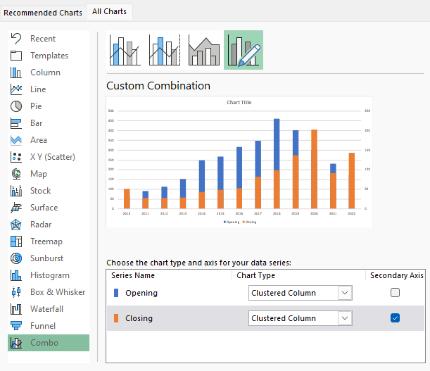
This is how you might normally look at these values when using column charts. But this time, I want the orange columns to be within the blue ones. Before I merge them together, I’m going to put the other chart on a secondary axis by right-clicking the chart and selecting Change Chart Type. At the bottom, I select Combo and make sure that they are both set to Clustered Column with the Closing series set to the Secondary Axis:
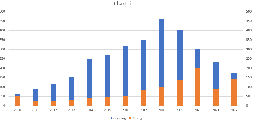
You can see that there is already a bit of an overlap in the charts. But the problem is that the axis have different ranges. To fix this, I’ll click on the secondary axis and select Format Axis. I will adjust it so the maximum value is set to the same as the maximum for the initial axis — 500. After doing that, my chart now looks like this:
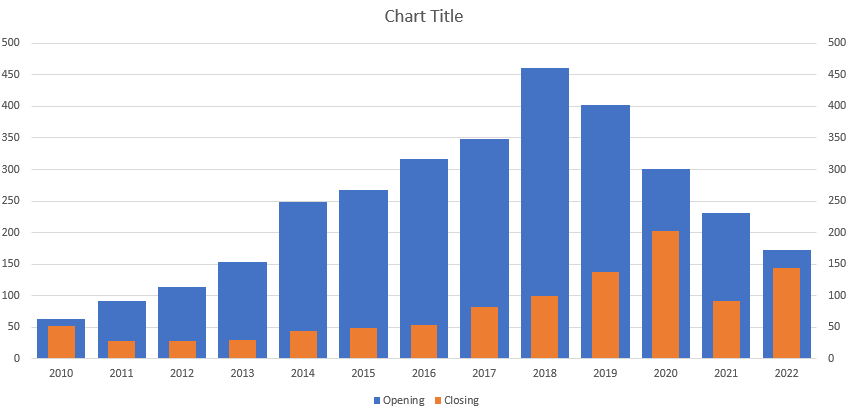
This is already getting close what I wanted initially. However, I still want to have more of an embedded effect, for the closing series to be within the opening series. Now, if I right-click on the blue column chart and select Format Data, I’ll have an option to modify the Gap Width. What the gap width does is shrink the amount of white space between the columns. After setting it to 25, it looks like this:
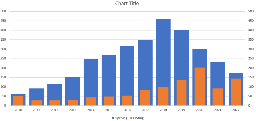
Next, I’ll set the orange columns to a gap width of 80:
The only thing left is possibly changing the color. To show that the two items are related, I prefer to use colors that are similar, with one being a darker shade than the other. I’ll also change the secondary axis font to white so that it is not visible, and add some vertical gridlines. That leaves me with this end result:
If you liked this post on How to Create a Column Chart Within Another Column Chart, please give this site a like on Facebook and also be sure to check out some of the many templates that we have available for download. You can also follow me on Twitter and YouTube. Also, please consider buying me a coffee if you find my website helpful and would like to support it.
In the fast-paced world of investing, identifying trending stocks in Excel can provide a valuable edge for investors seeking profitable opportunities. Fortunately, with the power of Excel’s Power Query and the ability to connect to a website’s API, accessing real-time data and uncovering trending stocks has become more accessible than ever. In this article, I will go through the process of using Power Query to connect to a website’s API and importing in trending stock information.
Why should investors try to identify trending stocks?
As an investor, it is crucial to identify trending and popular stocks for several reasons:
Profit Potential: Trending and popular stocks often have significant profit potential. When a stock is gaining popularity, it usually attracts more investors, leading to increased demand and potentially driving up the stock price. By identifying these stocks early, you can position yourself to benefit from the price appreciation and generate higher returns on your investment.
Liquidity: Popular stocks tend to have higher liquidity, meaning there is a larger pool of buyers and sellers in the market. This liquidity allows you to enter and exit positions more easily, ensuring that you can buy or sell shares without significantly impacting the stock’s price. Investing in liquid stocks provides flexibility and reduces the risk of being unable to execute trades at desired prices.
Market Validation: The popularity of a stock often reflects positive market sentiment and investor confidence. When a company is trending and gaining attention, it may indicate that the market believes in its growth prospects and overall performance. By identifying such stocks, you can align your investment choices with market sentiment and increase the likelihood of investing in companies with strong fundamentals and future growth potential.
InformationAvailability: Popular stocks generally attract more media coverage, research reports, and analyst attention. This increased coverage provides you with a wealth of information and analysis to make more informed investment decisions. You can leverage these resources to understand the company’s financial health, competitive position, industry trends, and other relevant factors that can impact the stock’s performance.
How to get trending stocks in Excel
To get trending stock data into Excel, you should start with finding a good source that you can rely on for trending data. For this example, I’m going to use apewidsom.io, which provides free access to its API using the following url: https://apewisdom.io/api/. Here’s how I’m going to use that to pull in trending data:
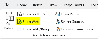
Extract the data using Power Query. To get started, I’ll select the Data tab in Excel and click on the From Web option.
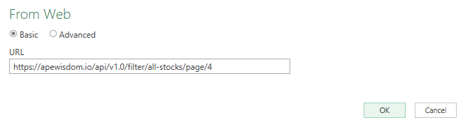
Next, there will be a field to enter the URL, this is where I will paste the link that the API references:
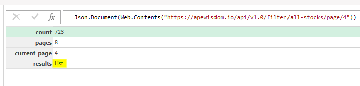
After clicking OK, Power Query will launch. When the screen opens up, the following table appears. I click on List to open up another table.
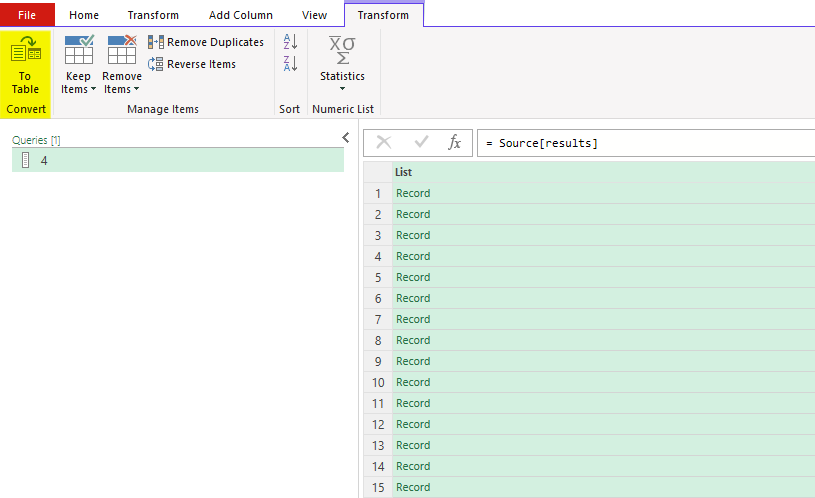
After clicking that, there’s another list of records.
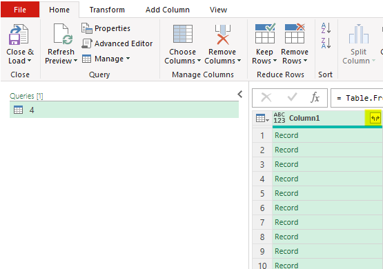
Here, I’ll select the option to convert to table and leave the default settings and click OK. Then, there is another list of records. Clicking on the button with the arrows going in opposite directions will expand them:
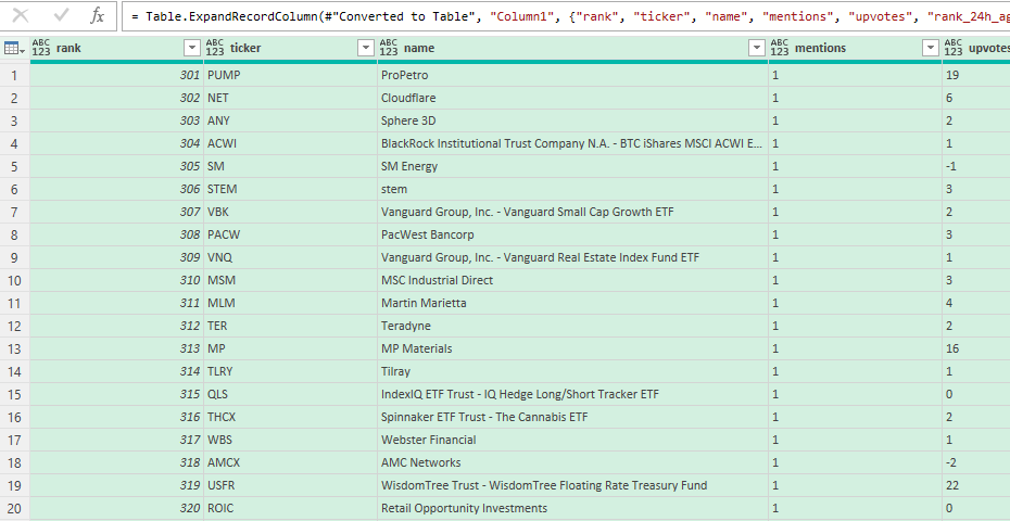
After expanding out those records, the table will now looks like a list of stocks and metrics relating to mentions, upvotes, and overall rank popularity:
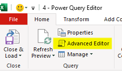
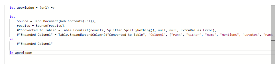
Now that this has been setup, I will convert this into a Power Query function. To do that, I’ll click on the Advanced Editor button:
In the editor, I will add a line at the top to specify the name of the function. And at the bottom, I will add a line to circle back to it. Lastly, I’ll add a variable for the URL as well, and put that where the link used to be:
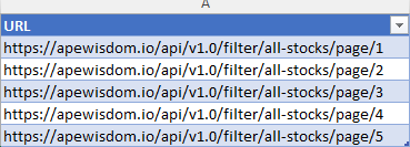
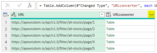
Next, with the custom function created, I’m going to go back into Excel and create a list of all the URLs I want to use this function on. In this situation, I’m going to adjust the page number at the end of the URL so that I have pages 1 through 5:
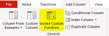
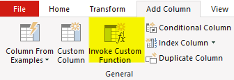
I’ll load this table, called URLtable, into Power Query using the From Table/Range button when selecting data. Next, I’ll select the Add Column tab and select Invoke Custom Function:
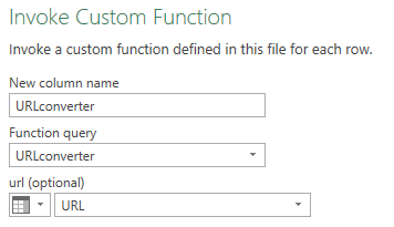
Then, I reference the query as well as the URL variable that is to be used:
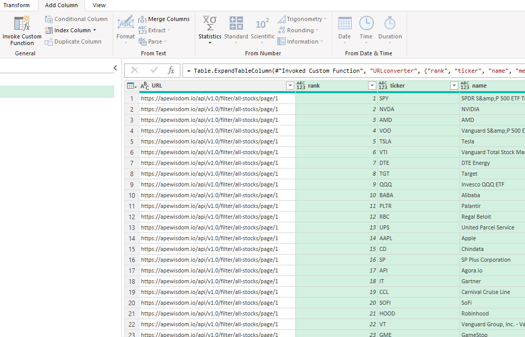
Then, there will be a field with the results, in table format. Again, this needs to be expanded out:
That will leave a list of stocks starting from page 1 all the way through page 5. You can remove the URL field, which is no longer needed:
If you don’t want to follow through all those steps yourself, you can download the template I’ve created here.
If you liked this post on Get Trending Stocks Into Excel Using Power Query, please give this site a like on Facebook and also be sure to check out some of the many templates that we have available for download. You can also follow me on Twitter and YouTube. Also, please consider buying me a coffee if you find my website helpful and would like to support it.
Excel’s Power Query is a powerful data transformation and analysis tool that allows users to retrieve, clean, and shape data from various sources. While Power Query provides an extensive set of built-in functions, there may be scenarios where you need to perform custom operations on your data. This is where custom functions in Power Query come into play. In this article, I will go over how to create a custom function in Power Query that you can invoke and re-use.
Steps to creating a custom function in Power Query
Creating custom functions in Power Query involves using the M language, which is the scripting language underlying Power Query. It can be complicated to create but I’ll show you two ways you can create a function. The first method is directly through coding, the other is after converting a query into a function.
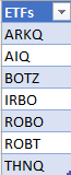
In this example, I’m going to pull all the stocks that are contained from a list of exchange-traded funds (ETFs). I’ve created the following table for this purpose, called tblETF:
Creating a custom function from scratch
If you’re creating a function in Power Query directly from code, here’s how to do that:
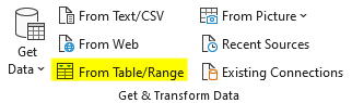
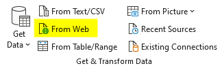
1. Go to load the data into Power Query by selecting a cell in your table, then click on the Data tab and click From Table/Range.
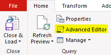
2. That will open up Power Query. Once there, on the Home Tab, click on the Advanced Editor button:
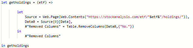
3. Create a name for the function using the let variable. In this example, I’m going to call it getholdings and it will pull all the holdings from the etf field. The opening line of the code is as follows:
let getholdings = (etf) =>
4. Next, list the commands that the function should execute. I’m going to pull the data from the stockanalysis.com page relating to the etf. This requires using the Web.Contents function and modifying the URL so that it includes the etf symbol:
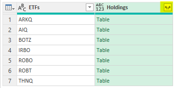
5. Now that the function is created, go into the query for the list of ETFs. Create an additional column from the Add Column tab, and select the button to Invoke Custom Function.
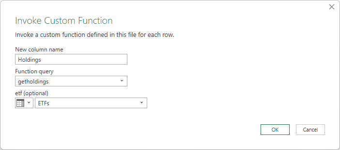
6. Set a column name for the new column. Then, specify the function query to reference. And you’ll also need to specify where the ETF value is coming from, which involves selecting the column:
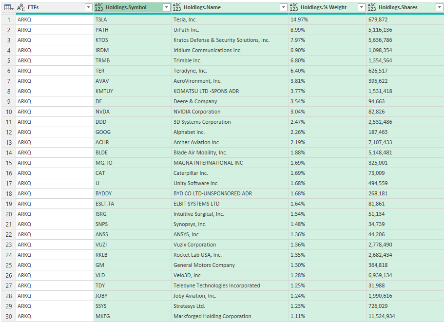
7. Next, you’ll expand the table that has been created within the column. This is done by pressing on the icon that shows arrows going in opposite directions. Then, select all the available columns.
You should end up with something that looks like this:
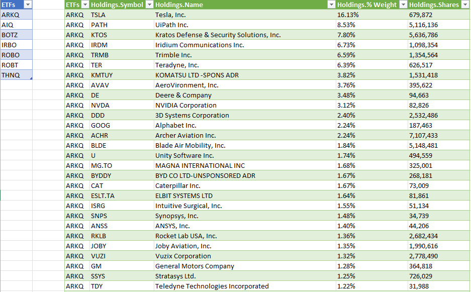
You can now click Close & Load and this data will load in your Excel spreadsheet. Now you can add to your ETF list and refresh the data, and the table of all the holdings will populate.
Converting a query into a function
If you’re not comfortable coding with Power Query, you can first create the steps, and then convert the query to a function.
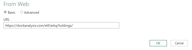
First, it’s necessary to create the query. In the previous example, I loaded the URL from a dynamic web page. To do that, I’ll start with selecting the From Web button on the Get & Transform Data section:
Next, populate the entire link, without the ETF variable — this will be added later:
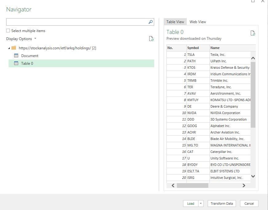
Then, select the table that contains the data and click the LoadTo button and select connection only:
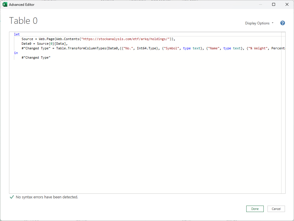
Then, right-click on the query to edit it so that you’re back in Power Query. From there, click on the Advanced Editor and you should see this:
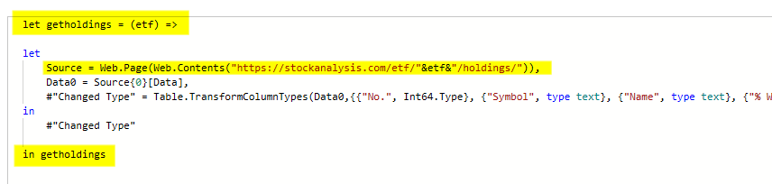
This is similar to the code in the first approach. To convert this into a function, we need to add another let variable and specify the function name, and any variables that will be used in the function. For the first line, I’ll add the following
let getholdings = (etf) =>
and for the URL, I’ll put the etf variable into there:
Here’s the updated code, with the changes highlighted in yellow:
Now I’ve converted my query into a function that can be invoked.
If you liked this post on How to Create a Custom Function in Power Query, please give this site a like on Facebook and also be sure to check out some of the many templates that we have available for download. You can also follow me on Twitter and YouTube. Also, please consider buying me a coffee if you find my website helpful and would like to support it.