Creating a Stock Screener in Excel

A stock screener allows you to filter through stocks that meet your investment criteria. It can help you find undervalued stocks and great dividend investments. But sometimes it can be cumbersome to always go back to a website and re-apply filters, even if you save them. In this post, I’ll go over how you can populate a list of stock data into Excel and then run your own filters on it, and thus, creating a screener you can easily access from within your own spreadsheet.

Step 1: Populating the list

The one thing you’ll want to do before you can create the screener in Excel is to download an array of stock data from a database. Personally, I like using Barchart because it has lots of useful information on there and you can get a wide range of data, and it is easily downloadable into an Excel format. It lets you do five free downloads each day and you can download 1,000 rows at a time. That’s thousands of stocks you can add. Using that in conjunction with the STOCKHISTORY function, and you can create a pretty versatile template. After all, since data like earnings, dividends, and other fields won’t often change, downloading a snapshot from Barchart once a month or even less frequently shouldn’t be a big issue. You can obviously use other databases but I’m going to use a free example for the purpose of this post.

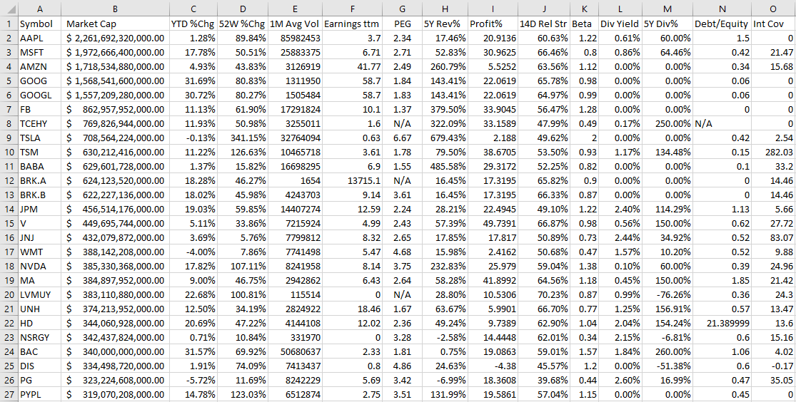
On Barchart, I’ve customized the fields I want to use for my downloads, and this allows me to re-use them again and make subsequent downloads easier. To keep it simple, I am going to download just the top 1,000 North American stocks based on market cap. This is what my download looks like in Excel:

Now that the data is loaded, the next step is to create the layout.

Step 2: Organizing the stock screener and setting up the fields

I find it most convenient to always put any inputs on a spreadsheet on the top of the page, and the results below. This way, you can freeze panes to make it easy to scroll through all the rows while seeing your selections.

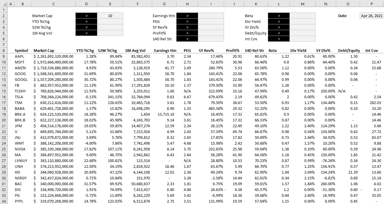
To start, I will create a field for each major field I have downloaded. After formatting some of my values, this is how my screener looks thus far:

Off to the right, I’ve added a date field because I am going to utilize Excel’s STOCKHISTORY function to pull in the price. This will allow me to calculate the current price to earnings ratio without having to download it from the screener as that multiple will change every day based on the stock’s price.

When downloading so many stock prices, it may take a while for the formulas to update. But once they are loaded, then I can calculate the P/E ratio by just taking the stock price and dividing it by the earnings per share.

Step 3: Creating the formulas to evaluate the criteria

The part that will take the most time is to now evaluate each of the criteria to determine if a stock meets all of it and whether it should be included in the results. Rather than trying to do this in one large formula, I’m going to break this up into one formula per field. I’m going to name these fields exactly the same so that it is easy to reference them.

For the first criteria, Market Cap, my formula looks as follows:

=IF(E2=””,TRUE,IF(D2=”>”,C9/1000000>E2,C9/1000000<E2))

D2 is where I have the dropdown for the > or < symbol and E2 is the value that I want to filter for market cap. C9 is the first row of data. My goal here is to evaluate to either a TRUE or FALSE value. I also divide the value in C9 by 1,000,000 just to make it easier to filter the market cap by millions.

For the % change calculations, I will do a similar calculation. Except this time I don’t need to divide by 1,000,000 and so it looks a lot simpler:

=IF(E3=””,TRUE,IF(D3=”>”,D9>E3,D9<E3))

D3 is my > or < dropdown while E3 is the percent change I am entering. Since I will enter a percentage here, I don’t need to make any special calculations. This is the same format that I will follow for the other fields.

Once I have set up all my calculations for the various criteria, I’m going to add one column that will check to see if the stock meets all of them. This is a simple formula where I can multiple all the values. A TRUE value will compute as 1 and a FALSE will be 0. And so even if there is one FALSE value, the entire result will return FALSE and not meet the criteria. The formula looks as follows:

=(T9*U9*V9*W9*X9*Y9*Z9*AA9*AB9*AC9*AD9*AE9*AF9*AG9)>0

Step 4: Converting it into a table

The final step is a simple one but it’s also important to make this sheet work smoothly. Select anywhere on the data set and on the Insert tab, click on Table. Hit OK and now you should see Excel’s default table applied to your data.

The reason for converting this into a table is that now we can apply slicers to it. And really, only one is needed here. If you go to the Table Design tab, there is a button to Insert Slicer. Click on it and select the one for the field that checks all the other criteria. In my example, it is called Criteria Met.

After hiding all the criteria fields, changing some of the formatting and adding the slicer, this is now how my screener looks like:

The beauty of this stock screener is that by clicking on the TRUE button in the slicer, you are automatically refreshing the data in Excel and updating your filters based on the selections. All this is done without macros and it makes the screener easy to change with the press of a button.

You can download my completed template here. Please note that if you do not have STOCKHISTORY available on your version of Excel, some of the values will not populate.

If you liked this post on creating a stock screener in Excel, please give this site a like on Facebook and also be sure to check out some of the many templates that we have available for download. You can also follow us on Twitter and YouTube.