stockhistorytemplate4

Stock History Template

Several weeks ago, I discovered that Excel had a new function called STOCKHISTORY. It’s able to pull stock prices and a great way to track stock prices and can help calculate returns. Excel does make it clear that it is not for trading purposes. However, it’s still a great way to stay on top of tracks and see how they’re performing. Below, I’ve created a template that will allow you to track stock prices and arrange them from best-to-worst.

Note that for this template to work, you need to have the STOCKHISTORY function on your computer, otherwise you’ll get nothing but errors. So your first step will be to check if it works on your file. Refer to the original post on the function as it will also explain how you can get it on your computer if you don’t already have it. If you’re running on old versions of Excel, you’re out of luck.

But for those that aren’t and that have access to the function, read on.

Using the template

You can download the template here.

There are three main inputs on this template:

  • Selecting the stocks you want to track.
  • Setting the date ranges you want to look at.
  • Entering the ranges that you want the macro to sort.

Let’s start with the first one, selecting stocks. I’ve already created three stock sections in this template, which you can of course change. Let’s look at one of them as an example:

List of stock prices on Excel.

The Start, End, and Return values are formulas. The only things you need to enter are the ticker symbols. Off to the left, shaded in light grey, I’ve also entered the code for the exchange. For the New York Stock Exchange, it’s XNYS, while the NASDAQ is XNAS. For a full list of the codes, refer to the original post on the STOCKHISTORY function. If it’s a popular stock that’s on one of the major exchanges, you may not need to enter it. I’ve included the exchange code for the sake of avoiding errors as it’s possible Excel might not know which ticker you’re looking for and select the wrong one.

You can extend the ranges to accommodate more tickers, you’ll just need to copy the formulas down in the Start, End, and Return sections.

Next: the date ranges.

Off to the right of the template, there’s a section where you can enter the start and end dates.

Start and end dates for the template.

The template will adjust for weekends but not for holidays. If you see a #VALUE! error in the values, that likely means there’s an issue with the date, so you’ll just need to change one of the dates to ensure it doesn’t fall on a holiday.

Lastly: the ranges to sort.

To the right of the dates, there’s another area where you can enter which cells to sort:

Cells to sort section.

Cells E8, K8, and Q8 on this template are where my ‘RETURN’ headers are located, and where the percentages are. If you add sections or modify this template, you’ll need to update the cells to sort. When you update the start or end dates, the template won’t automatically re-sort until you click on this button:

Re-sort button on the template.

If you get an error on the re-sort button, make sure you check which cells are in the Cells to Sort area and ensure that they’re correct.

#CONNECT! errors

One thing you may run into on this template are #CONNECT errors. I’ve noticed this happens once you start adding too many ticker symbols. Sometimes it’s hit or miss and you’ll get all the prices updated, but if you’re planning to list every ticker out there, just be forewarned that you might run into issues here. It’s a separate error from the #VALUE! error and one that can’t be fixed through the template, without removing some ticker symbols, anyway.


If you liked this post on the StockHistory Template, please give this site a like on Facebook and also be sure to check out some of the many templates that we have available for download. You can also follow us on Twitter and YouTube.

stockhistory

How to Use the New Stock History Function in Excel

For a while, one of the big advantages Google Sheets had over Excel was the ability to pull stock quotes easily. But that’s no longer the case as there is a new function in Excel that allows you to pull in stock price history. Below, I’ll cover how to use the StockHistory function.

How the function works

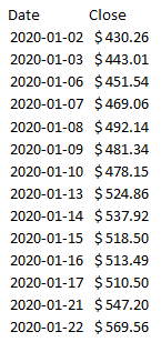
The function itself is fairly simple and requires just two arguments at a minimum, and that’s the stock ticker and the start date. By default, the function will return the closing prices from the start date until today. For instance, if I want to pull Tesla’s share price since the start of the year, this is what my formula will look like:

=STOCKHISTORY(“TSLA”,”2020-01-01″)

The formula will then generate an array. Here’s a portion of what it looks like:

Stockhistory function returning Tesla's share price since the start of the year.

If you want to pull just the most recent share price, here’s what you can do:

=STOCKHISTORY(“TSLA”,WORKDAY(TODAY(),-1))

Using the WORKDAY formula you can ensure that you’re going back one business day. You may need to adjust this if you’re on a weekend but basically you just need to manipulate the date to make this work. Note that this doesn’t appear to give you the current day’s close. When I ran this on a Friday, the most recent closing price it returned was from Thursday’s close. It’s clear this function’s intended for historical data rather than live or even delayed stock prices.

If you want to specify an end date for your data, you can enter a date in the third argument, right after the start date.

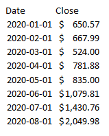
The function gives you many options, including which data points you want to pull in and what intervals you want. You can pull prices on a monthly or weekly basis by selecting either a 0 (daily), 1 (weekly), or 2 (monthly) for the interval argument. Here’s how I’d pull monthly prices for Tesla:

=STOCKHISTORY(“TSLA”,”2020-01-01″,,2)

Tesla's monthly share price since the start of the year.

It’s important to note that these aren’t monthly averages, they’re just the stock prices as of the end of the specified month. Although the date for the first entry suggests January 1 (the markets weren’t open that day), that’s actually the January 31 closing price.

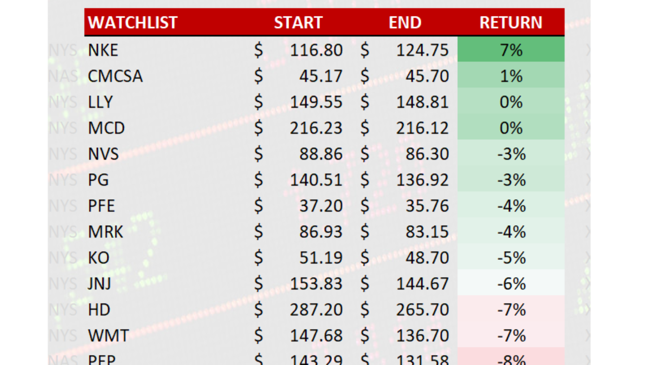
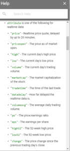
You can choose whether you want to see the headers and you can also add more fields, including the opening price, the high, the low, and the volume. You can even determine if you want to even see the date (although that’s probably not a good idea when you’re looking at historical data).

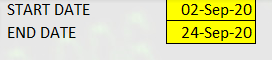
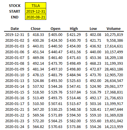
It’s easy to make a template with this function since it populates the data for you. Using variables for the ticker, the start date, and the end date, I can quickly set up a sheet that’s easily updatable:

Excel template using the stockhistory function.

The only formula that I enter is the one cell for the STOCKHISTORY function:

=STOCKHISTORY(C2,C3,C4,0,1,0,1,2,3,4,5)

Where C2, C3, and C4 refer to the stock, start, and end dates. The numbers 1 through 5 are needed to ensure that all the fields are extracted.

If you want more details about this function including the different arguments, you can check out Microsoft’s official page for this function.

How can I get other (non-US) tickers?

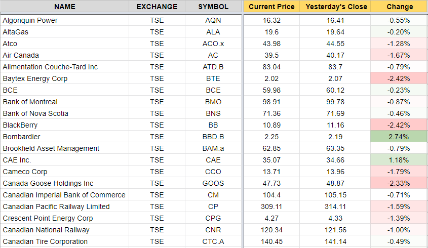
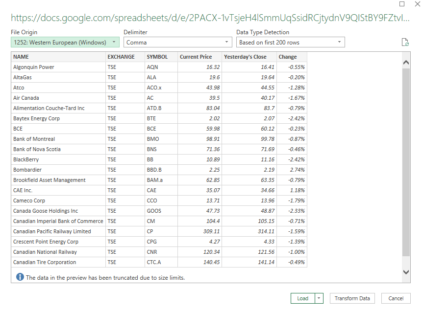
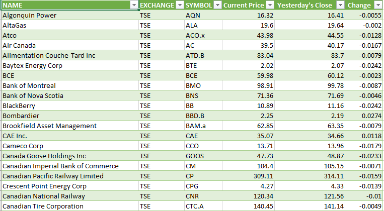
One of the things you’ll notice from the above examples is that I didn’t enter any prefix for the stock ticker. The StockHistory function knew I was looking for Tesla’s stock price. However, if you want to pull data from other exchanges, including those outside the U.S. markets, you’ll need to add a prefix to make sure that you’re getting the right quote. And since the function won’t actually return the company name, you need to make sure you’re entering the ticker correctly into the function.

Refer to this link for all the different market identifiers. For instance, if I wanted to pull the share price of Air Canada, which trades on the Toronto Stock Exchange, I’d need to enter the ticker as follows:

XTSE:AC

In most cases, it looks as though it’s just an X before the exchange’s usual prefix but you’ll want to double check to make sure.

Why you may not find the StockHistory function on your version of Excel

Since the function’s in beta, StockHistory is not available for most users. You can, however, sign up for Microsoft’s Office Insider program which will give you access to functions while they’re in beta. To join the program, follow the steps outlined here.


If you liked this post on How to Use the New Stock History Function in Excel, please give this site a like on Facebook and also be sure to check out some of the many templates that we have available for download. You can also follow us on Twitter and YouTube.

Average Down Calculator

Scroll further down if you would like to see details as to how this calculator works and a description of it.

There is a new version of this calculator available here (mobile-friendly) that will make calculations at multiple price points at once (use the new interval field to specify how much in price you want to jump by). It will also let you know how low you can average down at the current share price.

Also, be sure to check out this free average down calculator template in Excel.


Average Down Calculator

Amount Invested
Shares Owned Today
Current Average Price
Current Share Price
Desired Average Price

The purpose of this calculator

If you invest in stocks and want to know how much it would cost you to average down, this calculator will help you do just that. Averaging down is a great way to take advantage of a stock that’s dipped in value and that you’re confident won’t stay there. By purchasing more shares of a stock at a lower price, you’re bringing down the average cost of your total investment. And that means you’ll need the stock to rise to a lower price than before to turn a profit. Or if you’re already in the black, then you can put yourself in a great position to increase those profits.

How the average down calculator works

To use this calculator, you’ll need to enter the total dollars that you’ve invested in a stock, how many shares of it you own, what the current price of the stock is today (or the price that you plan to buy it at), as well as what price you want to average down to. Then, click on the Calculate button. The calculator will then tell you how many shares you’ll need to buy and how much it will cost you in order for you to get to that average.

Note that since you can’t average down below what the current share price is, you’ll have to make sure that your desired average price is higher than where the stock is today. Here is the calculator:


If you liked this free average down calculator, please give this site a like on Facebook and also be sure to check out some of the many templates that we have available for download.

Compounded Annual Growth Rate Calculator

If you don’t want to calculate compounded annual growth rate yourself, you can do it quickly and easily with this free calculator:


Calculating Compounded Annual Growth (CAGR)

Percent Change
Number of Years


[WP-Coder id="1"]

white-male-2064876_640

How to Add Stock Quotes Into Your Excel Spreadsheet

Unfortunately, there’s no Excel formula that can add stock quotes for you. However, there is a workaround for that which can help you get what you’re after. In a previous post, I covered how to pull stock quotes using Google Sheets which is able to pull in prices and all sorts of other data. And in this post, I’ll show you how to get the data from Google Sheets into Excel.

In essence, Google Sheets is your data source or database, and you’re going to import that into Excel. It’s not specific to stock quotes, but it’s an example of how you can accomplish the same thing. So first up, you want to create your file in Google Sheets using that earlier post as a guide. Here’s an excerpt of what my file looks like in Google Sheets:

google sheets stock prices

Once you’re ready, it’s time to link your Excel file to that Google Sheets file, and here’s how to do that:

How to Link Google Sheets to Excel

  1. On the File menu, click on the button to Publish to the web
publish to web google sheets

On the next screen, you should see something like this:

publish to web google sheets

2. Select the tab that you want to export under the Link section and change Web page to Comma-separated values (.csv) and click on the Publish button, that will generate a URL:

publish to web google sheets

3. Copy the URL that was generated in Step 2 and go back into Excel and under the Data tab click on the From Web button which is in the Get & Transform Data section

excel import google sheets

Paste it into the next screen’s URL field and click OK

import excel google sheets

On the next page you should see a preview of your data and if it looks okay then click on the Load button.

import excel google sheets

What you should see afterwards is what was on your Google Sheets tab from earlier:

import excel google sheets

And there you have it, your data from Google Sheets linked into Excel. If you make changes to your Google Sheets file, or if you want to refresh the stock quotes, right-click anywhere in the Excel sheet and select Refresh. Note that sometimes it may take some time before the file is updated on Google Sheets and before you’ll see any changes that you have made to the file.

It may not be an ideal solution if you’re looking to get stock quotes, but it gets the job done and avoids you having to try and find a complex formula or macro to pull the data that you want. You can use the Excel sheet with your Google Sheets data as a database and then lookup the stock prices from another sheet. The benefit of using Google Sheets is that you can have the best of both worlds – putting data online that you can easily update, and not be limited to Google Sheets and be able to edit and manipulate it as you need to in Excel.

Word of caution: if you delete or move around data in Google Sheets it could cause issues, especially if columns are missing and when you go to refresh it cannot find them anymore. If there is an error as a result of it or if you need to change the source, you’ll want to edit the query. When you click on the data in Excel you should see a section for Queries & Connections where you can edit the query. This is where you can select which data you want to include as well as change the source that you are pulling from. However, if it may be easier to just re-publish the data.


If you liked this post on How to Add Stock Quotes Into Your Excel Spreadsheet, please give this site a like on Facebook and also be sure to check out some of the many templates that we have available for download. You can also follow us on Twitter and YouTube.

google sheets start page

Use Google Sheets to Track Stock Prices and News

google sheets start page


One of the advantages of using Google Sheets over Excel is that it is easier to access live, dynamic data that you can access from any device that can install the app.

Pulling Stock Quotes


A great feature of Google Sheets is that you can easily pull stock prices (delayed) from Google Finance. There is a unique function called GOOGLEFINANCE that can pull any of the following stock details including price (including open, high, low), volume, even the last time it traded. If I wanted to pull Alphabet’s stock price I could use the following formula:

=GOOGLEFINANCE(“GOOG”,”price”)

That will pull me the most recent stock price. If I wanted to see the percent change since the last day’s close I would just change price to changepct:

=GOOGLEFINANCE(“GOOG”,”changepct”)

If you access the help you will see a list of more options:
But you can go even further than that, pulling multiple dates at a time. For example, if I wanted all the closing prices since the start of the year I would enter the following formula:


google sheets help


=GOOGLEFINANCE(“GOOG”,”price”,”Jan 1, 2017″,today())

In Google Sheets it automatically creates a table of values for you and you don’t have to worry about making an array like you would in Excel. The result of the above formula looks like this:

google sheets googlefinance function stock prices


I only entered the formula in cell A1 and it produced the list of results. You can also select an interval if you don’t want every day in the range to show a total.

Getting News Feeds Using RSS


Another unique function of Google Sheets is you can pull news feeds from your favorite news site using the IMPORTFEED function. The key thing is you need to find the rss feed of the news site you want. Finding this is as easy as typing the name of the news feed you want and rss after it. For example, the the list of all of CBC’s rss feeds are found on http://www.cbc.ca/rss/index.html. I can use the top stories rss feed of http://rss.cbc.ca/lineup/topstories.xml for my feed.

My formula in looks as follows:

 =IMPORTFEED(“http://rss.cbc.ca/lineup/topstories.xml”,”items title”)

By using “items title” it will only pull the title of the story, which is a bit neater and easier to look at as the titles do not take up as much space as the descriptions as well. If I selected “items” then I would get five columns of data – title, author, link, date, and the description.


Instead, what I can do is in the next column over enter the same formula and select “items url” which will now have the story and the related link next to each other. This way I can pick and choose what I want. This is how it would look:

google sheets importfeed news


I have shrunk down column A since I didn’t want the whole url to show.


I now have all the pieces to make a start page using nothing more than a spreadsheet:

google sheets startpage


Perhaps it doesn’t rival MSN or Google’s home page but it works for me. I’ve made the formulas for the stock calculations relevant to the cells in column B so I can change the ticker symbol as I want to. The main benefit with using this is 1) you don’t need to open a browser to get stock quotes or news, and 2) you can easily access this information from your phone, all you need is the Google Sheets app installed.

 But wait, that’s not all!

Translating Text

I’m not sure why Google felt the need to, but you can even use their translator function as well inside of Google Sheets using the GOOGLETRANSLATE function.

What I could do is translate these news articles. You need to know the two character code for the language, to get that you can find it on this website:

 https://sites.google.com/site/tomihasa/google-language-codes

So what I am going to do is translate the news headlines I pulled earlier and translate them into Chinese. Google has two language codes for Chinese – Simplified, and Traditional. I’ll go with simplified, which is zh-CN.


My formula looks like this:

=GOOGLETRANSLATE(B1,”en”,”zh-CN”)

My output looks like this:

google sheets googletranslate translate
So now you can pull news stories from your favorite news site (just figure out the rss link) and you can translate it into whatever language you want. Unfortunately I can’t tell the accuracy of the translation, ‘Simplified’ Chinese didn’t make it any simpler for me. I still can only make out CSIS from all of that translated text.