If you do a lot of driving and you need to expense it for tax purposes, then you know you need a good log to keep track of it. That’s what the mileage log template will help you do. Along with tracking all your trips, it will let you do the following:
Track both kilometers and miles and convert back to a base unit. So if you travel outside of the country and don’t want to do the conversions yourself, you can enter them as either kilometers or miles and the spreadsheet will convert it into your base unit.
Allow you to categorize statuses based on whether you are going to be reimbursed by your company or not.
Track both personal and business travel so you have a complete picture of all your mileage
A summary tab to help you see your mileage by month
How the template works
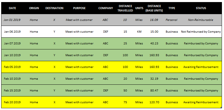
In the Log tab, simply enter the details from columns A through to J. There are drop-down options for units, type, and status. These drop downs can be changed from the Setup tab. If you need to add more lines to the table, look for the next empty row and in column A enter a date. The table will automatically expand.
The template currently is set to fit onto one page in landscape, but you can adjust the columns as you need. If you do not need to see the status and would just prefer the template goes until column I, then you can delete column J and all the conditional formatting will go away along with it.
Summary of the mileage log
On the Summary tab, you’ll see a breakdown by month of all the different statuses and km/miles traveled. This makes it easy for you to see how much mileage you still have to claim versus how much has been reimbursed for. If you delete the status column then you’ll of course not see this information and simply have the totals.
Customizing the mileage log template in the setup tab
On the Setup tab, you can make changes to the travel type. For instance, you could put a vehicle description in addition to whether it is personal or business. There’s no limit to the number of options you can have in this field.
In the status section, in the description field I’ve indicated what color a status will be highlighted in. If you want to change the name of the status, column C is where you can rename it.
In column G, you specify whether you want your base units to be in KM or miles. This will be used to convert the mileage and determining whether a calculation is needed. If you select miles as your base unit and on the log you put in KM for the units, then it will do a conversion back to miles on the log.
Download options
Feel free to test out the mileage log template by downloading the trial version here. The limitations of the trial version are that the setup tab is not available and it also has an advertisement.
If you’ve tried the trial and would like full version, please visit the product page here.
When you’re doing financial analysis, it’s helpful to add some context to growth numbers. That’s where using a Compounded Annual Growth Rate (CAGR) is very useful. Rather than saying a company has grown 50% over 10 years, you could say instead that they’ve grown by an average of 4.1% every year. It also gives you a percentage to use going forward if you need to forecast what you expect next year’s growth to be since you’ll have a starting point. The CAGR effectively tells you what the average growth rate has been during that period of time. It doesn’t mean that it’s grown every year by that rate, but that on average, it has risen by that amount. Below, I’ll go over how to calculate CAGR in Excel.
Using Amazon as an example
To calculate CAGR what you need to know are just two things: the total growth and the duration of time. Let’s use Amazon’s sales as an example. In 2018, total revenues for the year reached $233 billion. Back in 2010, the company had $34 billion in sales, meaning that Amazon’s revenues have grown by 585% during that time. Impressive, no doubt, but it doesn’t tell us how well it’s typically done on a yearly basis. This is where we calculate CAGR to help determine what the average growth was over that time.
From 2010 to 2018, that’s eight years that it took for sales to grow by 585%. To calculate CAGR, we use the following equation:
(Current Year Amount / Base Year Amount) ^ ( 1 / # of Years)
In the Amazon calculation, it would look as follows:
(233/34) ^ (1/8) – 1 = 27%
What this tells us is that Amazon for the past eight years has averaged an annual growth rate of around 27.2%. There’s an easy way we can prove this out. Starting with our base year of 2010, take the sales amount of $34 billion and multiply it by (1 + growth rate) each and every year. Here is how the level of growth looks like year over year:
Year
Prior Year Revenue
Growth
Current Year Revenue
2010
$34, 000
2011
$34,000
27.2%
$43,248
2012
$43,248
27.2%
$55,011
2013
$55,011
27.2%
$69,973
2014
$69,973
27.2%
$89,006
2015
$89,006
27.2%
$113,215
2016
$113,215
27.2%
$144,008
2017
$144,008
27.2%
$183,177
2018
$183,177
27.2%
$233,000
As you can see, if we assume a 27.2% growth rate each and every year, we arrive to the same end value. Although Amazon did not grow at this consistent of a pace, using CAGR helps to average the results over a period of time.
Whether you’re looking at sales, dividends, or any other kind of growth, using CAGR can be a very useful tool in putting into context just how the strong the rate of growth was.
Using CAGR to help forecast
Having CAGR is also useful if we want to forecast out future sales. Let’s assume that Amazon will have a more modest rate of growth for the next 10 years. That rather than a CAGR of 27.2%, it’ll be closer to 20% instead. Now, we can create a forecast around that and assume that sales will grow by 20% each year (on average) for the next 10. Our forecast would look as follows:
Year
Prior Year Revenue
Growth
Projected Revenue
2019
$233,000
20%
$279,600
2020
$279,600
20%
$335,520
2021
$335,520
20%
$402,624
2022
$402,624
20%
$483,149
2023
$483,149
20%
$579,779
2024
$579,779
20%
$695,734
2025
$695,734
20%
$834,881
2026
$834,881
20%
$1,001,857
2027
$1,001,857
20%
$1,202,229
2028
$1,202,229
20%
$1,442,675
To prove this out, what we can do is the following: 233,000 x (1.20^10) = 1,442,675
Based on these projections, we would expect amazon to hit the one trillion dollar mark in sales by the end of 2026. Maintaining a CAGR of 20%, however, will be difficult, even for a company like Amazon. Although all it takes is some big acquisitions and it will be well on its way!
If you don’t want to calculate CAGR on your own, you can use our free online calculator!
If you liked this post on How to Calculate CAGR in Excel, please give this site a like on Facebook and also be sure to check out some of the many templates that we have available for download. You can also follow us on Twitter and YouTube.
If you’re looking to hire someone and want to know whether they know how to code in Excel using Visual Basic (VBA), it’s not too hard of a task to quickly evaluate whether they know it or not. The first step is to ask them to send you a sample of something that they’ve done that includes coding and that is not password protected.
Then you’ll want to test to see what it does. So you’ll want to ask how it works so you can see for yourself. If that code works and the macro does what it’s supposed to do, you might be thinking that will be enough. However, someone could simply use a macro recorder to try and generate the code. This is not the same as coding and anyone can do this with no knowledge of code whatsoever. But there’s an easy way to uncover this.
Finding the code
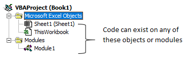
In the file that someone’s sent you, hit ALT+F11. This will send you into Excel’s backend and open up VBA. You should see something like this on the left-hand side:
Double click on each of those items – sheets, workbook, and any modules. Code can reside in any and all of those areas so you might need to cycle through to see where it is.
Once you find the code, that’s when you can start evaluating it.
Reviewing the code
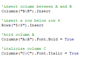
Below, I’ll show you the same macro, how it might look in VBA compared to how it looks using the macro recorder:
coding using VBA
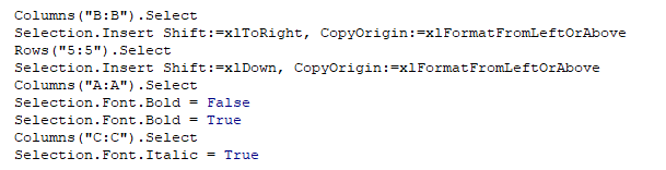
using the macro recorder
There are three things that should be clear from comparing the two examples above, which will help to identify whether someone’s just using the macro recorder or whether they’re actually coding properly using VBA.
1. Organization and spacing.
The macro recorder doesn’t care for spacing out the code and each line of code will come after the other. Especially when you’re looking at longer lines of code, it’ll get real messy real quick. Organization is important because if it looks like one big block of text it’s going to make it very difficult to audit or review later should you want to make changes.
2. No comments.
In the first example, there were lines in green that started with an apostrophe, called comments. They are optional but it ties back to the organization and putting notes along the way to help remind you what you were trying to do. It doesn’t have to accompany every line, but if you don’t see any comments at all, it could be a hint that someone just used a recorder. For a quick macro that’s only a couple lines long it probably wouldn’t be necessary, but for a lot of code you would certainly expect to see at least some comments.
3..Select.
In the second example, you’ll notice .select showing up multiples times. This makes it obvious that someone’s used the macro recorder. If you want to insert a column or bold it, you can just code it right away, you wouldn’t need to actually select it and then make the change. The macro recorder, however, records everything, including those selections. So seeing this should tell you right away that someone’s just used a recorder rather than coding it themselves.
There are other ways you could see whether the macro recorder was used or not but these three should suffice in helping you identify whether someone knows how to code or not.
Why does this matter?
If someone knows how to use the macro recorder, that’s good, but it’s not knowing how to code. The problem is that the macro recorder could do a small fraction of what is possible through actual coding. Coding through VBA opens up a lot more opportunities for automation and improving a spreadsheet. A macro recorder can be used by anyone but it lacks the sophistication to build much logic into it.
Knowing how to copy and paste is one of the most basic things you can learn to do in Excel. And while everyone is familiar with doing it, you might be surprised that there are several ways to do it, some more common than others.
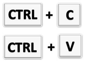
Using Ctrl + C and Ctrl + V
This is definitely one of the more common ways that people are familiar with copying and pasting. It simply involves selecting the cells you want to copy, pressing Ctrl + C, and then selecting where you want to paste them, and then clicking Ctrl+ V.
Using the mouse to right-click copy and paste
Also another one of the more common ways to copy and paste. Here you’ll select what you want to copy, right-click and select copy. Then, select where you want to paste the data, then click right-click and paste. This way avoids having to use the keyboard but requires pulling up the menu with two mouse clicks.
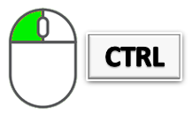
Using the mouse and keyboard together
Hold down Ctrl while selecting the cell that you want to copy and drag it to your destination. Then, release the mouse button and your data will be copied.
Note, if you release the Ctrl button first, and then release the mouse button, then you will have moved the cell (the equivalent of Ctrl + X, Ctrl+V) instead of copying it. The advantage of this method is you don’t have to click as much and it’s useful if you’re quickly copying within the same area. The disadvantage is this method won’t work if you want to copy the data onto another tab or workbook.
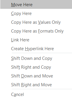
Using right-click to copy and paste
Select a cell and hover over the borders until you see a crosshair appear. Then hold down on right click and drag it to where you want to copy it to, then release the button. You’ll be left with many options, including copying the cell or moving it. Technically this involves a second click, but you only have to bring up the menu once.
Using VBA
This is obviously not a method I’d suggest if you wanted to just copy cells over one time unless it was part of a larger macro you’re working on. But to copy data over in VBA it’s a fairly straightforward process that includes just one line of code:
Range(“A1”).copy Range(“A2”)
The first range (A1) is the cell you’re copying and in the above example, A2 is where you’re pasting it to.
If you liked this post on How to Copy and Paste in Excel (5 Different Ways), please give this site a like on Facebook and also be sure to check out some of the many templates that we have available for download. You can also follow us on Twitter and YouTube.
If you’re looking for a way to compare worksheets in excel and find the differences between them, then this is the template for you. It will quickly highlight any changes between the worksheets and also note the differences. With just a push of a button and it being stored in the Ribbon, the macro is quick and easy to run.
How the Template Works
The steps involved in this template are fairly straight forward and to compare worksheets in excel becomes very easy. Simply open up this file and copy the sheets in that you want to compare.
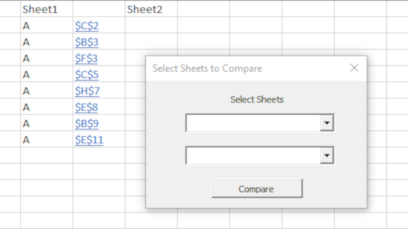
Then, on the Ribbon, select the Compare Sheets button.
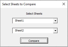
You will then be prompted to select which worksheets that you want to compare.
It’s important to note that when doing the comparison it isn’t looking at formatting and simply looking at the actual values.
Once you’ve selected the tabs you want to compare, click on the Compare button and the macro will run and will now compare worksheets. If you want to compare thousands of rows then this process will take a while and you’ll need to be a bit patient, since the macro will look cell by cell.
Before running the Compare Worksheets template
Important: If you’re not sure how big your data set is, use the CTRL + END shortcut, this will take you to the end of your data.
This is a good double check before you run the macro since you’ll get an idea of just how many rows and columns it’s going to look at. Sometimes the range is a lot bigger than expect since you might have many empty rows and columns if you copied data in before and never shrunk down the range.
But if you’re good to go, then run the macro and it’ll compare the worksheets.
What the output looks like
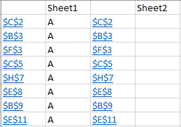
If there are no differences between the files, you’ll get a message box telling you that. Either way, the macro will end up creating a new sheet where it will plot all those differences. In my data sample, I put in a series of random A’s across the sheet:
As you can see, it’ll identify the individual cell as well as the value there, compared to the related cell in the other sheet and what value is there. It will also create a hyperlink so that you can go straight to that cell so that you can review it in case you want to dig a bit deeper.
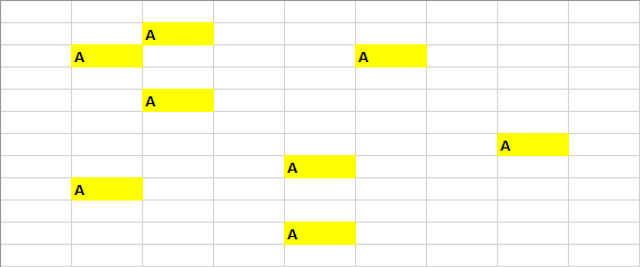
If you go onto the individual sheets that you compared, any differences from the other tab will be highlighted in yellow and bolded as well. This is just another way to tell you the cell is different than what’s on the other tab.
Sheet 1
Sheet 2
And that’s all there is to it. You can re-run the macro for any sheets that are within the file, although you’ll probably want to delete the one that gets created to highlight any differences once you’re done with it.
Download the Compare Worksheets Template
Free Version: Limited to first 20 rows. VBA code is locked.
Full Version: No limitations and code is fully unlocked.
Whether you’re managing multiple deadlines, have a lot of tasks, or just have an odd schedule, this task manager template can help you manage all of that. Visually you can see what’s coming up and what still needs to be done. It’s a good way to organize and manage all your responsibilities.
How the Task Manager Template works
I’ve tried apps to track deadlines and tasks and none of them have ever done what I wanted them to do. And since I spend a lot of time in Excel, I thought I’d try to make a task manager template that can be a one-stop shop for managing all of that.
The task manager has four main tabs to it that I’ll go over in detail:
Calendar
Recurring Deadlines
Tasks
Team Calendar
Calendar
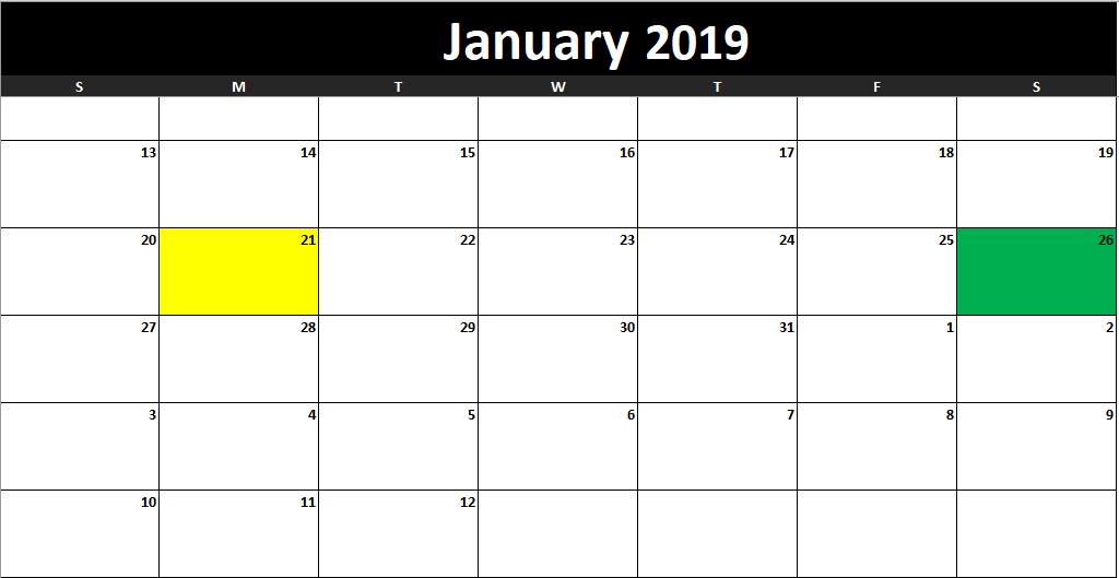
In its simplest form, you can use this tab to generate a calendar for whichever month and year you want just by changing the cell values. The calendar will highlight the current day as well as any holidays that you have specified.
It’s pretty simple, but once you start adding tasks and deadlines, it’ll look a whole lot different. I’ll refer back to the calendar as I go as it’ll change as I make updates to the other tabs.
Recurring Deadlines
There are multiple sections in this tab and it really acts as a setup tab, but the deadlines are definitely key.
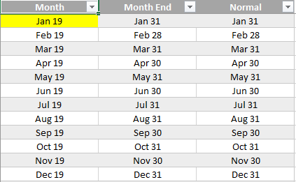
In the left-hand-side of the page is the month-end schedule. Now, if you’re not an accountant and don’t have to deal with month end, you can probably skip this. However, for accountants that deal with a close process and have deadlines, you can change the month-end date.
For example, I’m going to change the month-end date for January 2019 to February 12:
If I go back to the Calendar tab, even though I’ve selected January, the calendar will continue until February 12:
You can enter the month-end values for each month so that way each month will cut off where you want it to. If you don’t need a custom end to the month, then the default values will suffice and you they will just end when the month does.
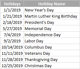
On the right side of the page there is a section for holidays. This is where you can put the non-working days in your part of the world. What you could also do is put any vacation days or time off that you have planned.
I’ve left a description of the holiday next to it but this is not necessary.
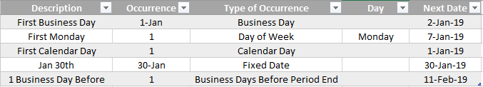
Now, if I go to the middle section of the tab, that’s where I see the recurring deadlines. There are five key fields here: description, occurrence, type of occurrence, day, and next date.
In the description field you’ll want to put in the name of the deadline. If you’ve got multiple deadlines on the same day you’ll want to combine them into one as they will only take up one line on the calendar anyway.
The occurrence and type of occurrence fields will go hand in hand. For example, if your deadline is the first business day of the month, then you’ll put a 1 in the occurrence field and Business Day in the type of occurrence.
If your deadline is the first Monday of the month, then enter a 1 in occurrence, Day of Week in the type of occurrence, and enter Monday in the day field (this is the only time you’ll need to use this field).
If your deadline is always the 1st calendar day of the month, then enter 1 for occurrence and Calendar Day in the type of occurrence field.
There’s an option to just enter a fixed date as well. If you always have a deadline on January 30th of every year, then enter the date in the occurrence field and Fixed Date on the occurrence type. This is helpful if you’ve got property taxes or annual deadlines that you can easily forget about. Of course, you’ll need to remember to update your deadlines.
Lastly, there is an occurrence type for Business Days Before Period End. Before your month end (whether custom or calendar), you can work backwards to compute your deadlines. Let’s say one business day before your cut off date you have to get a report submitted. In that case, you can enter a 1 for the occurrence and select Business Days Before Period End for the type.
Using the above scenarios, this is what my deadlines look like so far:
The Next Date field automatically gets populated based on what you’ve entered in the three prior fields.
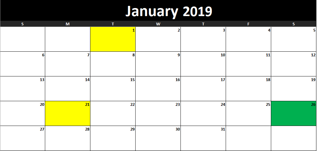
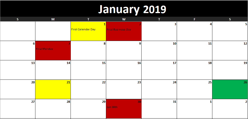
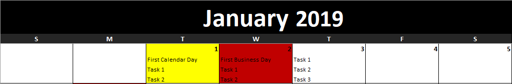
These deadlines now show up on my calendar:
The deadlines are highlighted in red (except where there’s a holiday, as on Jan 1). The description of the deadline also shows in the first line for that particular day as well.
Tasks
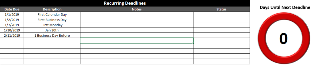
On the tasks tab, you’ll be able to see your deadlines, to do list, and tasks. In the first section, you see the deadlines which we’ve already entered thus far:
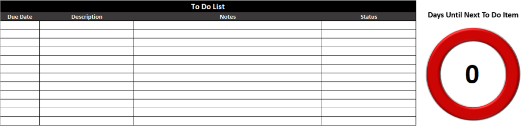
You can add any notes to this section as well as update the status of the deadline. If you haven’t completed deadlines that are in the past, the Days Until Deadline visual will show a zero. However, if I update the status to ‘Completed’ for all the tasks in the past, then my countdown will update to show many days until my next deadline:
This now gives me an accurate countdown as to how many days away I’m showing until the next deadline.
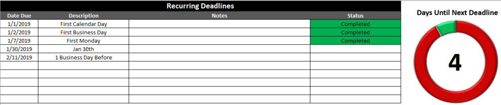
The To Do List won’t show up on the calendar and is just a way for you to track items you’re working on now. It will also show another countdown and is similar to how the recurring deadlines work in this section:
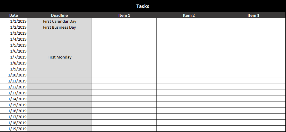
The last section on this tab is the tasks section.
This section is important since this is what will show up on your calendar. The deadline column will automatically be the first item on the list. And so you have a limit of three tasks that will show up on your calendar (two if there is a deadline there).
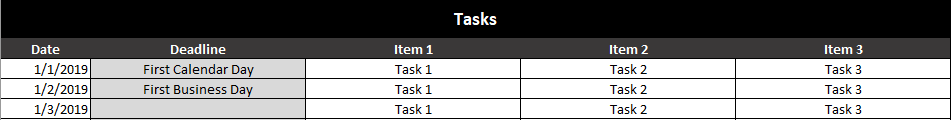
For the first three days of the year, I’m going to put the same three tasks:
This is how the calendar now looks:
Because the first two days of the year each had deadlines, only Task 1 and Task 2 made it onto those days. On the third day, all three tasks showed up.
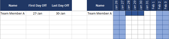
Team Calendar
If you’re working on projects or teams, you might find it helpful to have a glimpse as to when people are off.
On the left side of the page, you fill in the person’s name and the range of dates that they are off. You can enter in multiple ranges for the same person so the names can repeat.
Next to the actual dates, you’ll want to enter each person’s name that you wish to track (which I’d presume is everyone that is on the left side that you have entries for).
The date will automatically start at today and you’ll see the next 90 days of availability. Any holidays and weekends will be highlighted in light blue. Any time off outside of that will be highlighted in dark blue as in the above example.
Download the Task Manager Template
Free Version – Limit of 10 task and recurring deadlines, contains ads and sheets are locked.
Full Version – 30 recurring deadlines and to-do-list items. No ads and no sheets are locked.
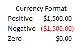
There are many different options for formatting data in a spreadsheet. And there are even more available if you use a custom number format in Excel. That flexibility is important because it can be a bit frustrating if, for example, you want negative numbers to show up with a dollar sign as you have to use the currency format in that situation — which does not look very polished:
The positive and negative amounts look okay but I’d like to see a bit more spacing. But the bigger issue for me is the $0.00 formatting which can create a lot of noise if you’re looking at financials with lots of zeroes over the place (although I have a solution for this). It can divert your attention away from what you want to see — the cells that have non-zero values.
Creating a Custom Number Format
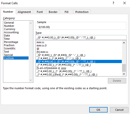
Although it may not be available by default, there is certainly a way to get a whole lot closer to the formatting that I want, and I’ll show you how. To start, you want to select the accounting format and then flip over to the Custom format (to do this right-click and select Format Cells). You’ll notice this is what the string looks like in the Type field:
This is what the accounting format looks like. The formatting is broken out into four main parts: positive, negative, zero, and text.
The string that appears until the first semi-colon is how the number will look when it is positive. Until the next semi-colon is the negative formatting, followed by if the value is zero and the last one is text.
Here is what the positive amount looks like in the accounting format:
_($* #,##0.00);(
The negative formatting looks very similar:
_($* (#,##0.00);
The main difference you’ll notice is the extra bracket “(” that is in the negative format. That is what puts the negative amounts in parentheses. Now, if I want to make this highlighted in red, all I would need to do is add [Red] right after the semicolon that indicates the end of the positive format:
($* #,##0.00);[Red]($* (#,##0.00);($* “-“??);(@_)
Upon doing that change, my number now comes up in red:
These are all the color options you can use:
Black
Blue
Cyan
Green
Magenta
Red
White
Yellow
There’s not any added customization you can do to these colors. And as you can imagine, many of these colors will be an eyesore on the default white background, and I’m not sure why you would even need to use the default black value. Blue, magenta, and red are the only ones that are easy to read and that won’t make you want to change the background color.
More Customization Options
For more complete customization, you’re better off looking at how to use conditional formatting.
If you need to make other tweaks to number formats what you can do is select the format and then switch over to the Custom section. Then you’ll see what that format looks like and you can test out what adjustments you’d like. Whether it’s adjusting the spacing or how the format looks like with a zero value, these are changes you can easily make and see what works through some trial and error.
If you’re interested in looking how to format dates, check out this post.
If you liked this How to Create a Custom Number Format in Excel, please give this site a like on Facebook and also be sure to check out some of the many templates that we have available for download. You can also follow us on Twitter and YouTube.
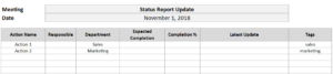
Excel can be a useful tool for tracking items, whether related to a meeting or a project. The action items template allows you to enter multiple fields related to an action item, including responsible person, department, expected completion, and tags to help organize them.
You’ll be able to create new action items, sort them into different department tabs, recall the ones you want when it’s a new meeting, update the items, and archive them when they’re done.
Let’s start from the beginning.
First, fill out all the fields relating to the action items from your meeting.
The tags field will help when you recall meeting items in case you only want ones related to sales, a project, or some other criteria. Tags can be separated any way you want – comma, space, or any other separator.
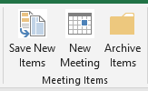
Then, click Save New Items, which will put them into every relevant tab.
By default, I have the sales and marketing tabs setup, but if you need more departments simply copy those tabs. If a tab doesn’t exist for the department, then you’ll get an error and it won’t be able to populate those tabs.
However, you don’t need to have a department for each action item and can simply assign a generic one.
The sales tab now shows the action item:
If a comment is left blank, then it will simply say ‘no update’ was made. In the comment field, it will always show the date of the meeting.
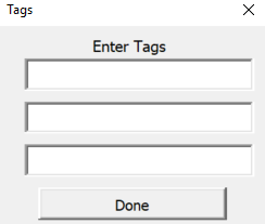
Now, say you want to make a new meeting and want to populate the action items. Click on the New Meeting button. This will give you the opportunity to enter any tags:
You can enter up to three different tags in your criteria. This is where if you have a specific type of meeting you can use the tags to help identify which items you want to populate in your meeting list. Of course, this assumes you entered the tag in the action item to begin with. If you do want to include everything, leave the tags blank and just click Done
When you pull up a new meeting it will only recall the most recent comment. Any items that show the completion at 100% will not populate the meeting items.
Any comments you enter now in the Latest Update field will add to the existing comments.
If you have items that are completed and don’t want to see them on the individual department tabs, you can click on the Archive Items button and that will move the items into the Archive tab.
Pivot Tables are great tools, especially for quickly summarizing data and allowing you to avoid entering in complex formulas to do so. However, they aren’t perfect and definitely have their quirks about them.
Here are four things that most users aren’t crazy about, and how to fix them.
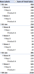
The layout
When you create a pivot table it puts the table into a layout that is less than optional for spreadsheets. It’s not only hard to use for any other purpose, but it’s also not the easiest format to read. I always prefer a format that resembles more of a spreadsheet itself, in a grid format, without the indented rows.
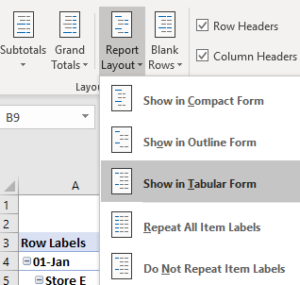
To change the format, go to the Design section of the PivotTable Tools and select Report Layout and select Show in Tabular Form
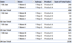
This is what the pivot table looks like after the change:
This might still look a little cluttered, but what you can also do is get rid of any subtotals by simply right-clicking on the Total and unchecking the Subtotal button, and then it’s a bit cleaner:
The table still needs a little work for me, and that brings me to the second issue:
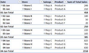
Labels do not repeat
You’ll notice that the value in the date field only shows up once. And so if I had many entries for a given date there would be a lot of blank values in the first column. Again, this is not ideal for a large data set and so this is where I’d like to make a change as well.
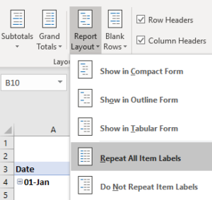
I go back to the Report Layout section, except this time I select the option to Repeat All Item Labels
Now my table looks like this:
This is what I would hope the pivot table looks like right off the bat. Unfortunately, Microsoft does not agree and opts for the indented version with subtotal at every section and no repeating values.
But that’s not all, there’s another little nuance you may notice when it comes to pivot tables:
Formatting won’t stay consistent
You’ll notice that in the sales data, I have a total of 2158 for January 4th. Anytime you’re dealing with numbers in the thousands, you’ll probably want some formatting that shows a comma in there just to make the numbers more readable. However, if you simply select the entire column and change the formatting, it will revert back to the default if you refresh the pivot table after adding more data.
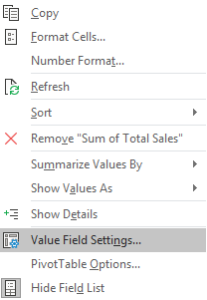
What you need to do is actually change the field settings. To do this, right click on any of the numbers in that column and select Value Field Settings.
From there, select Number Format and then select the format you want it to show up as. Doing this will ensure the formatting won’t change when you refresh the data.
Tip: if you routinely make these changes like I do, you may want to check out the add-in I created which will make all these changes for you at the click of a button.
This brings me to the fourth most irritating item when it comes to pivot tables:
GETPIVOTDATA
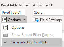
By default, when you reference a number in a pivot table, it will auto-generate a formula called GETPIVOTDATA. In most cases, you probably won’t find this helpful, especially if you just want to reference some pivot table values elsewhere in your workbook. If you just want to reference cell E4 and copy the formula down, you’ll need to adjust the pivot table settings, as the GETPIVOTDATA will make it a bit painful to accomplish this.
Back under the PivotTable Tools section, select the Analyze tab and on the Options menu on the left-hand side, uncheck where it says Generate GetPivotData
Now you can reference values from a pivot table the way you would any other cell in your workbook.
If you have any other frustrations with pivot tables, please share them in the comments.