Cleaning up data – getting rid of blank or 0 values in Excel

This function is designed to help clean up a spreadsheet if you want to either delete or hide cells that have 0 or empty values. How this works:

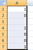
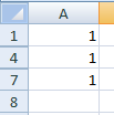
I select a range of data that I want to get 0s and blank cells out of (it doesn’t have to be a column) and run the macro.

The macro will hide everything that is a blank cell or a zero value in my range:

What if I only wanted 0s, or blank cells only? What if I wanted to delete the entire row that has that cell?

In the code below, you can change these options based on what you want the function to do. I have created two variables called option1 and option2. Their values are bolded in red.

If I change option1 from 1 to 2, then only 0 value cells will be affected, a value of 3 will mean only blank cells are.

For option 2 I can choose to hide the entire row (1), hide the entire column (2), delete the row (3), delete the column (4), clear the cells (5), delete the specific cells and shift cells up (6), or delete the cells and shift left (7).

Changing the values in red allows you to make any of the above changes.

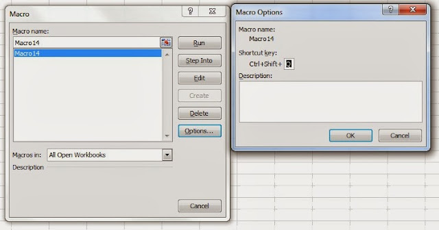
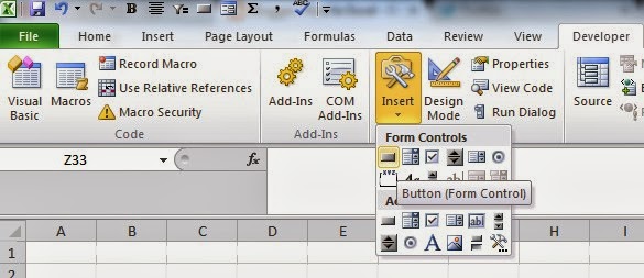
The code for the macro is below. I suggest assigning a shortcut for this macro to run it quickly.
———————————————————————————————————————–

Sub cleanupdata()

Dim option1, option2 As Integer

option1 = 1
‘Option1
‘1 = blanks and 0s
‘2 = 0s only
‘3 = blanks only

option2 = 1
‘Option2
‘1 = hide row
‘2 = hide column
‘3 = delete row
‘4 = delete column
‘5 = clear cells
‘6 = delete cell, shift up
‘7 = delete cell, shift left

Dim activerange As Range
Dim cl As Range
Dim selectedcells As Collection
Dim numberofitems As Integer
Set selectedcells = New Collection

Set activerange = Selection

For Each cl In activerange

Select Case option1

    Case Is = 1 ‘Blanks and 0s
            If Len(cl) = 0 Or (Len(cl) > 0 And cl = 0) Then
                selectedcells.Add cl
               
            End If
           
    Case Is = 2 ‘0s only
            If Len(cl) > 0 And cl = 0 Then
                selectedcells.Add cl
            End If
                     
    Case Is = 3 ‘Blanks only
            If Len(cl) = 0 Then
                selectedcells.Add cl
            End If
           
End Select
Next cl

numberofitems = selectedcells.Count

On Error Resume Next
Select Case option2
    Case Is = 1
        For counter = 1 To numberofitems
        selectedcells.Item(counter).EntireRow.Hidden = True
        Next counter
    Case Is = 2
        For counter = 1 To numberofitems
        selectedcells.Item(counter).EntireColumn.Hidden = True
        Next counter
    Case Is = 3
        For counter = 1 To numberofitems
        selectedcells.Item(counter).EntireRow.Delete
        Next counter
    Case Is = 4
        For counter = 1 To numberofitems
        selectedcells.Item(counter).EntireColumn.Delete
        Next counter
    Case Is = 5
        For counter = 1 To numberofitems
        selectedcells.Item(counter).Delete
        Next counter
    Case Is = 6
        For counter = 1 To numberofitems
        selectedcells.Item(counter).Select
        Selection.Delete shift:=xlUp
        Next counter
    Case Is = 7
        For counter = 1 To numberofitems
        selectedcells.Item(counter).Select
        Selection.Delete shift:=xlToLeft
        Next counter
End Select

End Sub

———————————————————————————————————————–

Convert LAST NAME, FIRST NAME into different formats

In many databases names may show up as last name, first name which doesn’t make it ideal for sorting and filtering data easily. However this can be quickly rearranged in Excel. I’ll show you two ways to do this: 1) using text to columns (the easier method) and 2) using formulas

1) Using Text-to-Columns

Select the cells that have the last name, first name format and under the Data tab click on Text to Columns.

On the popup that comes up select Delimited and click Next

On the next screen, make sure Comma is the only delimiter selected and then press Finish

Doing this will put the last names in the current range and the first names in the adjacent column B. You will want to make sure the adjacent column is blank to make sure you don’t accidentally overwrite data that may be in those cells already.

An optional step, if you wanted to combine both last name and first name into one cell is to use the following formula in cell C18:

=B18&” “&A18

B18 is the first name and A18 is the last name fields. The ampersand connects the words with a blank space inbetween. Cell C18 would show John Smith

For Excel purposes, it’s probably ideal to have the last name and first name in separate cells rather than in one.

2) Using Formulas

Extracting the Last Name

First, the formula to extract the last name (assuming the cell is A2):

=LEFT(A2,FIND(“,”,A2,1)-1)

If I have Smith, John in cell A2, then the result is as follows:

The LEFT function extracts x number of letters from the left of the cell. The key is the second argument. It consists of:

FIND(“,”,A2,1)-1

The FIND function looks for a comma within cell A2, and begins at the 1st character. If the cell is Smith, John then the comma would be found in the 6th character of that cell. The -1 that is after the FIND function is to reduce this to the 5th character. This is done because I don’t want to include the comma in the name.

So how the LEFT function works is from cell A2 it pulls the first 5 characters from the left, which will result in Smith

Had I not included the -1 after the FIND function, it would have been Smith,


Extracting the First Name

Now I’ll show you how to extract the first name using a similar function, the RIGHT function:

=RIGHT(A2,LEN(A2)-FIND(“,”,A2,1)-1)

The logic behind the RIGHT function is the same as the LEFT function, except this time the formula pulls the characters from the right instead of the left. However you’ll notice the second argument is a little more complex this time. The argument is as follows:

LEN(A2)-FIND(“,”,A2,1)-1

The key difference is I am now using the LEN function which tells me the number of characters that are in the cell. LEN(A2) would return 11 characters for Smith, John

Why can’t I just use the RIGHT function the way I used the LEFT one? The reason being is the FIND function searches from left to right and not from right to left, so it will tell me the position of the comma from the left, not from the right. So if it returns the number 6, I know the comma is the 6th character from the left, but doesn’t tell me how many from the right.

In order to do this I have to use the LEN function. If the total cell is 11 characters long, and the comma is at the 6th character, that will mean there are 5 characters after the comma. Coincidentally in this case the comma is 6 spots from both the left and right, making it right in the middle of the cell.

Here again I use the -1 after the FIND function because if I pull the 5 characters from the right, it will include a blank space (obviously if the data is formatted as last name,first name instead of last name, first name you can omit the -1).

Combining the Two

Now these two functions have allowed me to pull the different parts of the name out of a comma separated last name, first name format. If you want all of this into one formula (and assuming you want first name last name to be in a single cell) then all you would need to do is enter the formula as follows:

=RIGHT(A2,LEN(A2)-FIND(“,”,A2,1)-1)&” “&LEFT(A2,FIND(“,”,A2,1)-1)

I’m reusing the formulas used earlier and connecting them with ampersands while also adding a space inbetween.

Highlight Alternating Rows or Columns

This post will show you how to create the effect of highlighting alternating rows, which sometimes makes it easier to read a data set.

In order to accomplish this, first select all the cells in the worksheet and then select New Rule under conditional formatting.

For the new rule you will need to select the last option to use a formula. The formula we will need to use is as follows:
=MOD(ROW(A1),2)=1
The MOD function calculates the remainder after division and has two arguments, the number to be divided into, and by what number. 
Using ROW(A1) means the reference will change depending on the location of the cell, meaning it will encompass every row in the selection. Using 2 as the divisor will help identify if the row is as odd number or even. If you’d rather highlight columns than rows, use the COLUMN function.
The formula will be true if the remainder is 1, meaning the row is an odd number (e.g. highlighting will start on the first row). If you want highlighting to start from row 2, just change the 1 to a 0, since even rows will have no remainder.
Once the formula is set, click on Format to determine the appearance of the alternating rows.
I select a light blue colour for the alternating rows
After I press OK this is the result of my conditional formatting:
If you don’t want to apply the formatting to all the cells or want to change the range, under conditional formatting select manage rules
There you will see a field where the formatting Applies to. Here you can change the range you want the formatting to apply to.

Using Custom Functions and Macros

If you come across a custom function or macro that you want to use in your spreadsheets, this post will show you how to do so.

As far as coding goes, they key difference in a function as opposed to a sub procedure in Excel is in the way the code is executed. In a function, you enter in just like you would any other function, by typing out the name of the function and entering in any required arguments. With a sub procedure, it is typically executed via an event, a button, or shortcut key. Also with a function, the user will manually enter values for key variables, whereas for a sub procedure in most cases those will be calculated within the procedure itself.

I’ll demonstrate how a custom function works and how to copy it into your code.
Below is a basic function that will multiply a value by 5:
__________________________________________________________________
Function times5(multiply As Integer)
times5 = multiply * 5
End Function
__________________________________________________________________

If you came across this code and wanted to insert it into your spreadsheet, what you would do is open VBA (alt + F11). Once inside VBA, click on Insert and select Module


Now paste the code into that module
And that’s all you would need to do before you can start using a custom function. Now if I go back into a worksheet, I can begin using the code by using the name of the function in my formula.

 There is only one argument in my function that I have to enter, that is for the multiply variable. Inside the function times5 there is one variable declared (multiply). The formula multiplies the variable by 5 to arrive at the result. If I had multiple variables (e.g.if the first line read Function times5(multiply as integer, multiply2 as integer) then that would signify two variables that need to be identified) then I would need to enter more than one argument, the way you would for any other function in Excel that has multiple arguments. But in this case I only have one variable.
Now as you will see, the result is the multiply variable multiplied by 5.
I can access this function for any worksheet within this workbook. If you want to copy a custom function to your spreadsheet, follow the above steps and then you can utilize that function in your worksheets. 
The one downside of custom functions is that the tool tips that normally show up in regular Excel formulas telling you what arguments are required are not available and so you need to make a note of what arguments are required for a function.

Inserting a Sub Procedure (Macro)

If instead of a custom function you had sub procedure (macro) you wanted to copy into your code, the steps would be the same, except instead of using a formula to execute the code, you would need to assign either a shortcut key or a button

Referencing Cells in Other Worksheets and Workbooks using the INDIRECT function

When working with multiple worksheets or tabs, it becomes useful to reference them in formulas or to consolidate data. First, I’ll look at working with different tabs.
Referencing Other Tabs

The easiest way to refer to a cell in another tab is to start a formula with the = sign, and then click over to the other tab and click on the cell you want to reference.  In the following example I am typing a formula in tab A but will reference cell B6 on tab B.
Note the reference in the formula bar:
=B!B6
The tab is denoted by the ! after the tab name. If I wanted to reference tab A it would look as follows:
=A!B6
But what if my tab wasn’t all one word, and the tab was named A and B? In this case, I would need to use apostrophes:
=’A and B’!B6
So to summarize, the naming convention for referencing another sheet is:
SHEET1!A1 or ’SHEET 1’!A1


Linking to other Spreadsheets

Now let’s assume the cell you want to reference isn’t in this same workbook, then the reference looks a bit different. If the workbook is open:
=[Workbookname] SHEET1!A1

The key difference is you are adding the workbookname. This method will work if the workbook is open, but not recommended if you are referencing a workbook that is closed because Excel might not know which workbook you want to reference and cause errors. To properly reference a closed workbook, use the following:
=’C:Desktop[Workbookname.xlsx]SHEET1!A1
The above formula will work if the workbook is saved on my desktop.
In this example I only used a single cell, but you can just as easily reference a range. Change A1 to A1:A10 and you are referencing a range instead of a cell. This comes in useful if you want to use the reference in a lookup.
Using the INDIRECTFunction

Referencing other worksheets and tabs is not difficult once you get used to the syntax, but if you had dozens of tabs or workbooks you wanted to reference, it might get tiresome to keep doing this. That’s where the INDIRECT function comes in handy. You can use formulas to populate these cell references so that you don’t have to re-type them or even use find and replace.
Imagine you have sales data on multiple tabs. Each tab represents a year. So if I want to summarize data from five different years (tabs), that’s five different references I have to use. Or I can use the INDIRECT function. The way the formula works is you can enter the entire location of the cell that you want to reference. The benefit is being able to use relative and absolute references in place of having to type out the full address over and over again.
Here is a comparison of how the references would look using each method:
In the indirect function, I am able to use a relative reference for the year. If I enter the formula in cell B4, all I have to do is copy the formula down and it will reference all the other years(tabs) without having to re-type the full location. The benefit here is apparent when you are dealing with many different tabs. In column C I am unable to do this and have to re-key each cell individually.
The tricky part of using the indirect function is making sure you are correctly combining the ampersands, variables, and constants. The ampersand you use to join a constant and a variable within the INDIRECT formula. In this example, the variable is the year (tab name). The constant is the syntax (!) and the cell reference (A1), since their values will never change.  Never put the variable in quotations, only constants. 
Here is a breakdown of the logic of the formula in cell B4:
Because I am referencing another tab (not another workbook), I need to start with the worksheet name. Since I have a variable for the worksheet name, I start with the reference to cell A4, which contains the name of my worksheet: 
=INDIRECT(A4
The remainder of the formula is going to be !A1, or, the constants. To add the constants, I need to add the ampersand, open quotations, enter the constants, and close the quotations and the formula:
=INDIRECT(A4&”!A1”)
You can alternate between constant and variable as much as you like but they have to be linked by an ampersand. You also don’t need to begin the INDIRECT function with a variable, it can be a constant.
Using INDIRECT with Workbooks
You can use the INDIRECT function to reference other workbooks, but unfortunately a limitation of the formula is that it is unable to get data from a closed workbook. So unless you plan to have the workbooks open, the formula will not be of much help here. The formula is most helpful when dealing with multiple tabs in a single workbook.
Avoiding Errors

Some key things to remember when referencing other sheets or workbooks:
  • Syntax is important, like in all formulas, but in these cases it’s very easy to make an error. Remember the !  comes right before the cell reference, and in the case of other workbooks, ‘! precedes it.
  • The INDIRECT function will help expedite referencing other tabs, but cannot help you with referencing closed workbooks.
  • If your tabs do not follow a consistent, predictable pattern then a formula won’t be able to help you much
  • You won’t be able to get data from closed workbooks that are password protected
  • Don’t forget the extension. In my example it was .xlsx but it may be different depending on your version and type of file.

How to Create a Named Range in Excel

Naming ranges offers an easy way to refer to a single cell or range without having to remember the address, and instead referring to it by name instead. This comes particularly useful if you will continually be referring to that cell. 
The key advantages of using named ranges:
– Less time consuming to find a named cell
– Easier to put into formulas
– Easier to reference in VBA
– Easily inserting hyperlinks in documents

Creating Named Ranges


Below I have sales data listed by month. If I wanted to reference total sales I would need to refer to cell B14.
Let’s say this sheet is just one of many, and these are sales for product A.  The more products I have, the more useful it becomes to have named ranges, otherwise I would have to either a) remember the location when typing a formula, or b) navigating to the cell I want to reference. By using a name, it is easier to recall and doesn’t take much effort to include in a complex formula that may include many references.What I could do is name cell B14 as ProductASales (and subsequent ones could follow the same patter – ProductBSales, ProductCSales, etc..)
All I do is select cell B14 and type ProductASales in the cell reference that previously had B14. B14 still exists, but now I can reference the cell by just typing in ProductASales as well.
A range can have more than one name. If you want to delete or edit a name select the Name Managerunder the Formulas tab
I find that I have created two names for the same range. To delete one I just select the name I don’t want and click Delete. Now if I just wanted to change the range I can click Edit

There I can change the range to whatever I want.
Named ranges can also be used for multiple cells in the same way.

Note that a named range will move as a relative reference. If you insert or delete rows the name will move along with your cells. It can also expand, just like any other range in Excel. If for instance you insert a row between May and June, that will add that row to the range. Instead of including the cells from A2:B13, it will now include the cells from A2:B14 – since December will be pushed down to row 14.

Now that the ranges are setup, they can be referred to in a formula.

In cell H8 you can see that I entered a formula consisting only of the named range ProductASales. Instead of referencing cell B14 I can use this name.
This won’t work the same way for the Sales range since it relates to more than one cell. However, I can use it as part of a formula, vlookup for example:
Here I am using Sales as a table. Instead of typing out the full range A2:B13 I only have to type in Sales.

Apply Named Ranges to Existing Formulas


But let’s say you didn’t realize you could use named ranges and have been manually entering the ranges. You can update your formulas so they reflect the named ranges by doing the following:
Under the Formulastab, select Define Name, and Apply Names.
 At the following screen I select both names and press OK.
Now all my formulas with B14 or A2:B13 will be replaced with ProductASales, and Sales, respectively. This won’t affect your formulas in any way but now if you look at a formula you can easily see if it is referencing a named range.

Using Named Ranges in VBA


Another benefit of using named ranges is that it makes it easier to keep formulas consistent. In VBA, to reference these ranges, unnamed, would be as follows:
Worksheets(“Sheet1”).Range(“B14”)
Worksheets(“Sheet1”).Range(“A2:B13”)
The problem with this is that if you move the cells around, cut, copy, the references in VBA are absolute and will never update the way relative references in Excel will.  However, if you use named ranges, this problem is avoided. The reference would be as follows:
Range(“ProductASales”)
Range(“Sales”)
If you are coding in another worksheet, you will have to qualify which spreadsheet the named range is in:
Worksheets(“Sheet1”).Range(“ProductASales”)
Worksheets(“Sheet1”).Range(“Sales”)
Now if these ranges are moved within Excel, you don’t have to worry about updating them within VBA.

Named Ranges as Hyperlinks


By using a named range you can also easily add hyperlinks into your spreadsheet. For example, let’s say on Sheet 2 I want to link to the sales data:
On the Insert tab, select Hyperlink.
Select Place in this Document and you will see a list of the defined names. If I press Sales and click OK this will create a hyperlink in the active cell:
Now if I click on the Sales link in cell D6 it will bring me to the named range that belongs to Sales.

IF Functions: Calculating Data If Criteria Is Met

An overview of how various IF functions work

IF Function
An if function creates a test, and can have different results depending on whether the test is true or false.

Example 1

 =IF(A1=”A”,1,0)
In this example, if A1 is equal to the letter A then the result of the formula is 1. If it is equal to B, C, or anything else, the result will be 0. It will look for an exact match – if you don’t want an exact match, you’ll need to use wildcards (see later down).
You can make nested If functions as well – instead of putting  a 0 in the formula above you can add another if function:
Example 2

=IF(A1=”A”,1,IF(A1=”B”,2,0))
In this formula, if the cell A1 does not match A, then it will do another test. The second test is checking to see if it matches B – if it does, it will assign a value of 2, and if not, a value of 0. You can keep adding If functions as much as you need to. But keep track of the parentheses to make sure they are properly closed. If you find yourself having to do many nested if functions then you may be better off using a lookup formula.
COUNTIF Function
The COUNTIF formula counts the number of items your criteria is met. See the example below:
Example 3
=COUNTIF(A1:A7,”A”)
This formula is looking at all the cells in the range A1:A7 and counting them if the match the letter A. This would result in 5. 
In newer versions of Excel, there is a plural version of COUNTIF– COUNTIFS. This allows you to use multiple criteria:

Example 4

=COUNTIFS(A1:A7,”A”,B1:B7,1)
This formula builds on the last, where it looks for the value A in cells A1:A7 and then also looks for the number 1 in cells B1:B7. This would result in 2. As there are two instances where A and 1 are in the same row. 
Note: If your ranges are not identical (e.g. A1:A7 and B1:B6), your formula will not work properly. Also, because in this example the formula was looking for a number, it does not have to be in quotations. You can keep adding more criteria by adding another comma instead of closing the formula.
SUMIF
SUMIF function works similarly to COUNTIF, the difference being is it can sum a separate range:
Example 5

=SUMIF(A1:A7,”A”,B1:B7)
In this formula, it will add all the values in B1:B7 when the corresponding values in A1:A7 are equal to A. This would result in a value of 10 (1 + 1 + 2 + 3 + 3). Like the COUNTIF function, SUMIF also has a plural version SUMIFS that can be used for more than one criteria.
There is a minor difference in how SUMIFS works:

Example 6

=SUMIFS(C1:C7,A1:A7,”A”,B1:B7,1)
In this formula, the values in C1:C7 will be added when the corresponding values in A1:A7 are equal to A and the values in B1:B7 are equal to 1. The key difference here is you select the range you want to sum first, and then the criteria comes after. In the SUMIF function, the criteria range came first, and then the range to sum came after. Similarly to the COUNTIF function, you can keep adding criteria with additional commas.
AVERAGEIF
This function works the same was as sumif, the main difference is instead of summing everything, it will take the average:
Example 7

=AVERAGEIF(A1:A7,”A”,B1:B7)
This formula will take the average of all the cells in the range B1:B7 where the related values in A1:A7 equal A. Similar to the way SUMIFS works, so too does AVERAGEIFS.
WILDCARDS
The above examples worked well if you wanted to match exactly what was in the cell. But what if you needed only to match one word or letter, or a portion? That is where wildcards become useful.
The first way to use a wildcard, is by using an asterisk (*). An asterisk represents unknown values before or after. For example:
Example 8
=COUNTIF(A19:A28,”P*”)
In this example, it will count the names that start with the letter P. Because the criteria start with P and is followed by an asterisk, what this means is that the first letter has to be a P, and the rest can be anything (three cells match this criteria)
Similarly:
Example 9

=COUNTIF(A19:A28, “*P”)
This formula works the opposite way, in that it will count the cells where P is the last letter, and any values can come before (no cells meet this criteria).
And also:
Example 10

=COUNTIF(A19:A28, “*P*”)
This formula will count the cells where P is anywhere in the cell (the same three cells that matched Example 8 are the only ones true here as well).
Note: the criteria here is not case sensitive.
But what if you are only looking for a certain number of characters? For example:
Example 11

=COUNTIF(A19:A28,”*H???”)
In this formula, it will count names that end with the letter h and 3 characters after. The ? represents one character (cannot be a number). This allows you to control your result to a finite length, whereas the asterisk doesn’t limit the number of characters. The cells that meet this criteria are A21 and A27.
A similar formula:
Example 12
=COUNTIF(A19:A28,”E??c*”)

This formula will look in the range and count the cells that start with the letter e, have any two letters after that, then a c, and anything else after that. The only result in the list is cell A24.

Brief Intro to Macros and VBA

If you do a lot of repetitive tasks (and even if you don’t), macros can help save lots of time. In some cases you can be talking hours worth of work in one macro.

Recording a Macro

Now, if you’re not familiar with macros or VBA at all, a good way to learn is through the macro recorder tool (this is under the View tab in the ribbon). When you record your macro, you can see what was created on the VBA side by pressing ALT+F11 – you can also edit your macro here. You can do much more in VBA by coding straight from that screen, as the macro recorder is limited (e.g. it can’t create variables or other complex codes). But the macro recorder helps you learn how to reference different items.

When you create a macro – whether directly from VBA or the macro recorder, you can assign a shortcut (or a button to it) to it, saving you time in executing it.

To assign a shortcut: select the view macros option under the view tab and then select options for the macro you want. There it will allow you to assign a shortcut (see below)

For a button, you will need the developer tab enabled. If you don’t have it, go under Excel options and under ribbon options you will see an option to enable it.

Once enabled, under the developer tab you will see an insert controls button where you can insert a button (see below)

Once you do that you will create the size of the button, and when you are done it will ask you to assign a macro to it. And now when you click on that button your macro will run.

Inserting VBA Code

If you run across VBA code that you want to copy into your spreadsheet, you want to make sure it is put in the proper section.

If it is a custom function, you want to make sure that is put in a module to work properly. If you do not see a module section in VBA, you will need to add one from the Insert menu.

If it is just a macro (denoted by ‘Sub’ and then the name of the procedure) it can be put in a module, the worksheets, or the workbook section. If you want the macro to work in all worksheets, then I would recommend putting it in the workbook rather than the individual sheets.

Extracting Unique Values

For Excel 2007 and newer:

Select the data you want to extract unique values from, and under the Data tab, click on Remove Duplicates.

If the column you select is alongside other data, it will remove those cells as well. If that’s not what you want, I’d recommend copying the column over somewhere else so it is by itself, and then click on the Remove Duplicates button.

For Excel 2003 and older:

Run an Advanced Filter on the column that you want to extract duplicates from, leave the criteria Blank, select Copy to Another Location, and select Unique Records Only.

Note, select the advanced filter option when you are in the sheet you want to extract the values to. For example, if your data is on sheet 1 and you want to extract the duplicates to sheet 2, you need to select advanced filter while you are on sheet 2, otherwise there will be an error.

VLOOKUP vs INDEX and MATCH

Lookups are popular in Excel and here I’ll look at the more popular one – VLOOKUP. However it’s not always the best option for doing lookups in Excel, and I’ll show you why.

VLOOKUP
Exact Matches
What Vlookup does is look for a value you have selected, and if it finds it, will return a value from the same table that corresponds to the matched value.
One of the key limitations of VLOOKUP is it cannot return results left of the matched item, only to the right. This is where I recommend the INDEX & MATCH formula (see later down), as that combination will allow you to go left or right and won’t require you to re-arrange your worksheet just to accommodate a formula.
Example 1

If I wanted to lookup value B in the table, I would enter the following formula:
=VLOOKUP(A7,A1:D4,2,false)
This will equal the value in cell B2, the number 2. If I changed the column number from 2 to 3:
=VLOOKUP(A7,A1:D4,3,false)
It would return the number 22, or cell C2.
If I selected column 5, it would result in an error because my table range (A1:D4) only contains four columns.
If instead of looking up letters in column A I wanted to lookup numbers in column B, I would have to change my table range from A1:D4 to B1:D4, and it would look like this:
=VLOOKUP(A7,B1:D4,3,false)
I would also have to change the value in A7 so that it is a number. But again, if I change the formula this way I cannot move to the left and find out what letter corresponds to my value. Not without re-arranging my table.
Note that before I changed the range column 3 related to column C, now it relates to D because the table has shifted. Column 3 relates to the column number in the table, not in the spreadsheet.
                                                                                   
Approximate Matches

The one strength of VLOOKUP is determining what category or range a value falls into. By changing the last argument in the formula to true, Vlookup no longer looks for an exact match. Why would this be useful? Let’s say you have the first 3 letters/numbers of a postal/zip code. Because there are so many combinations possible, you would have to list each one out to find an exact match. 

With VLOOKUP’s approximate match, it will determine the closest match (e.g. shipping rate codes won’t spell out an entire postal/zip code, but will often cite a range). Similarly, if you have tax brackets and need to know what bracket an income level falls into, this is where it would be useful as well. The one caveat is that the values in the table must be in ascending order.
Hlookup is a parallel formula to Vlookup, only that it looks horizontally rather than vertically.
Example 2
In this example, my formula looks like this:
=VLOOKUP(A7,A1:B4,2,TRUE)
The argument at the end has changed from FALSE to TRUE, meaning an exact match is no longer needed. If I had set it to TRUE, it would return an error. But in this case, it returns cell B2, or 2. The reason for this, is because the values are in ascending order, it correctly identifies that V3A falls between V2B and V3C. Since it has not yet reached V3C, it belongs to V2B. If V3A is changed to V4D, X, Y, or a value greater than V4D, it will equal 4, as it will recognize that it belongs to the highest category.

INDEX & MATCH
I mentioned using INDEX & MATCH will give you a more versatile formula. This formula is structured differently than VLOOKUP in that it will pull the coordinates from the row and column number you specify. The match function will allow you to determine the proper row number based on your search criteria, and the column number you can decide – whether it is left or right of the matched value, it doesn’t matter here.
Example 3
Going back to the Example 1, I’ll show you how using the INDEX & MATCH formula will be able to now move to the left and pull values from column A:
=INDEX(A1:D4,MATCH(A7,B1:B4,0),1)
The range is unchanged, but the second argument in the INDEX formula (relating to row number) is calculated using the MATCH formula. The MATCH formula looks for the value in A7 (1), in the range B1:B4 and returns the row number. The 0 in the MATCH formula represents an exact match. After the MATCH formula, the last argument in the INDEX formula is the column number, which has been set to 1, which will return the values in column A. The advantage of using INDEX and MATCH as you can see is you can change the column number to 1, 2, 3, or 4. Similarly, if you wanted to look up the values in column C instead of B, you would change the formula as follows:
=INDEX(A1:D4,MATCH(A7,C1:C4,0),1)
In this case you don’t need to change the column number, it doesn’t move since you don’t have to rearrange the table.
In short, when you should use either formula:
Looking up a value – INDEX & MATCH*
Finding a value based on ranges – VLOOKUP
*unless you just want a quick formula and the values you need are to the right