If you have sales data organized by country, you can create map charts in both Excel and Google sheets. These charts can make it easy to visualize sales and identify patterns and trends. Below, I will compare the different ways to create map charts in Excel and Google Sheets, and highlight any similarities and differences.
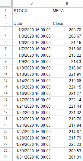
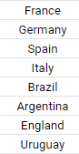
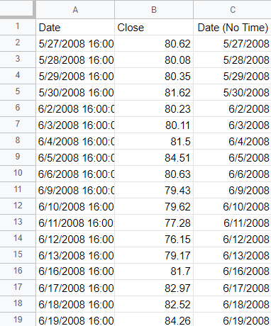
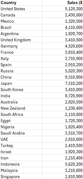
For this example, I’m going to use a data set which just includes two fields, one for the country and one for the sales data.
Creating a map chart in Excel
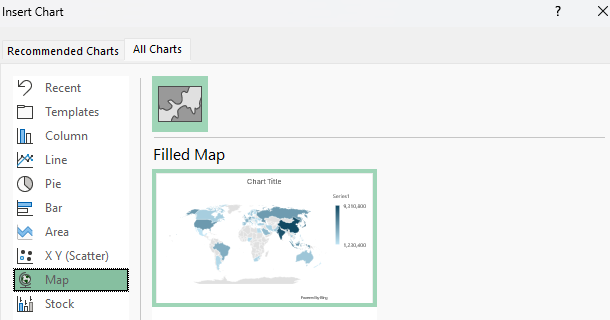
To create a map chart in Excel, all you need to do is click anywhere on your data set and insert a chart. Excel will likely automatically detect the data and recommend a Filled Map as an option. But if it doesn’t, you can select a Map option under the All Charts tab:
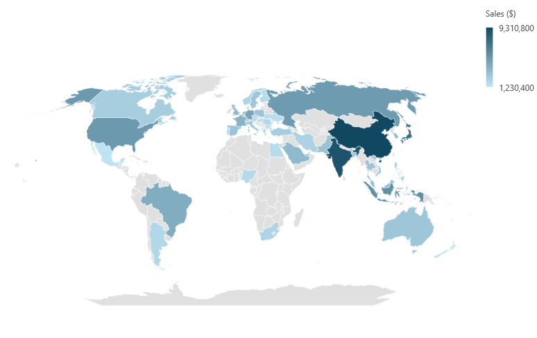
You’ll now have a chart that displays the values based on a color scale. In this example, the larger values are in a darker shade of blue whereas the smaller values are in light blue. And if there is no data, the countries are filled in grey.
As with other Excel charts, you can specify a different color scheme and chart layout. In the chart below, I’ve used a theme which has a black background.
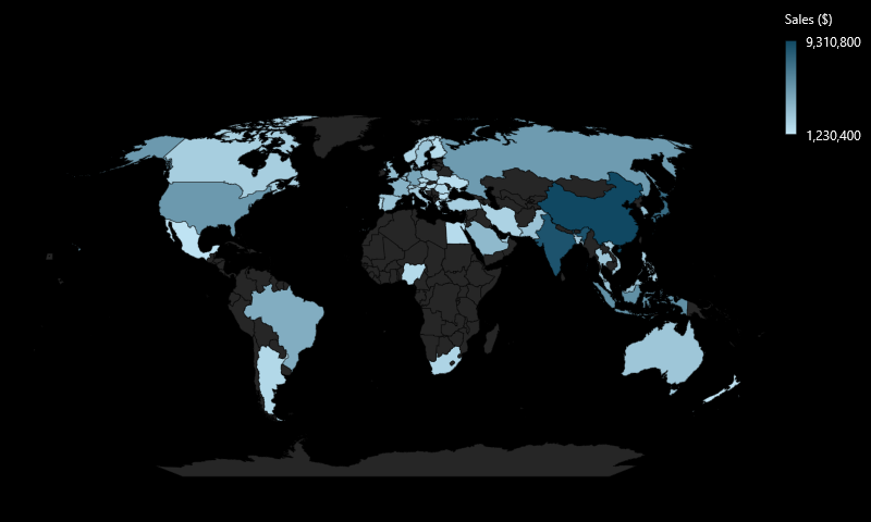
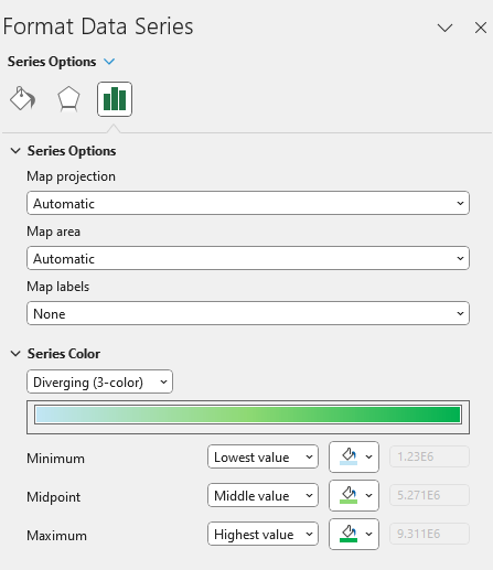
By using the dark theme, it makes it easier to focus on areas where there is data, as those countries stand out more prominently. You can also manually adjust the color scheme for the chart by formatting the data series. To do so, right-click on the chart, select Format Data Series and under the option for Series Color, you can specify a 3-color range. And you can adjust what the minimum, midpoint, and maximum values should look like. This logic is similar to how you might set up conditional formatting rules in Excel.
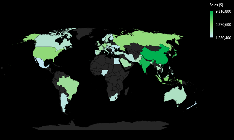
With more colors, readers can now see more variation in visualization.
Creating a map chart in Google Sheets
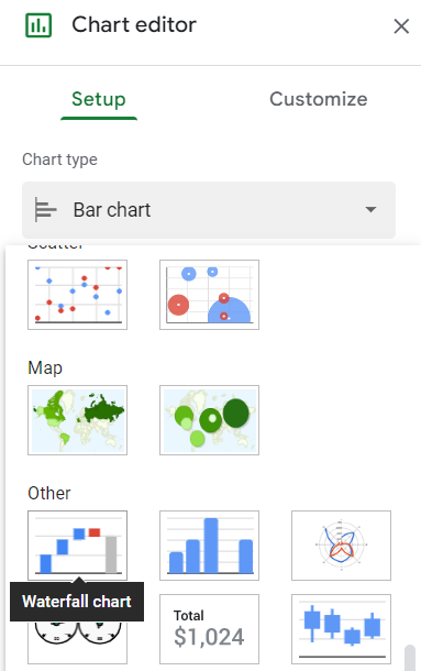
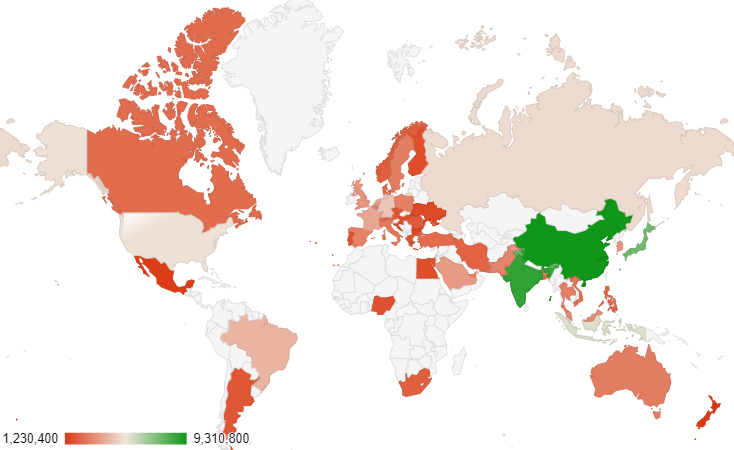
To create a map chart in Google Sheets, the process is comparable to Excel’s. Simply select a cell on your data set and when you create a chart, select the option for Geo Chart under the Map section
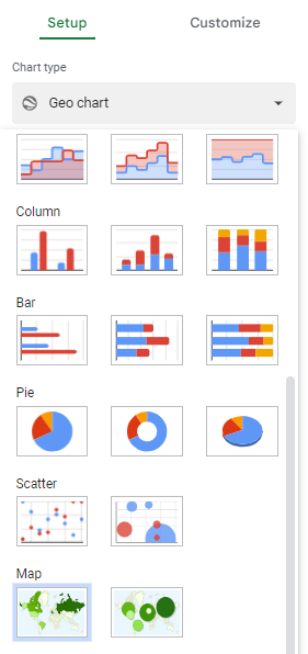
The result is similar to Excel, with the countries being shaded based on their values:
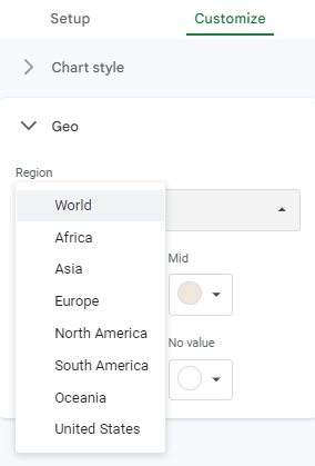
Under the Customize section of the chart settings, you can specify what the max, min, mid values should look like. In addition, you can specify how countries without values should be displayed.
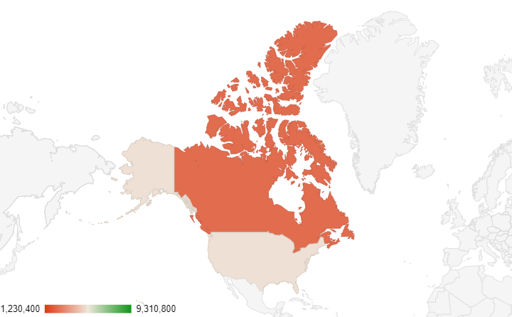
In Google Sheets, you also have a bit more flexibility in how to zoom in on data. In the region drop down, you can specify whether you want to look at the entire world, or narrow in on specific continents.
If I select North America, then I will only get a view of that continent, even if there is data for other countries.
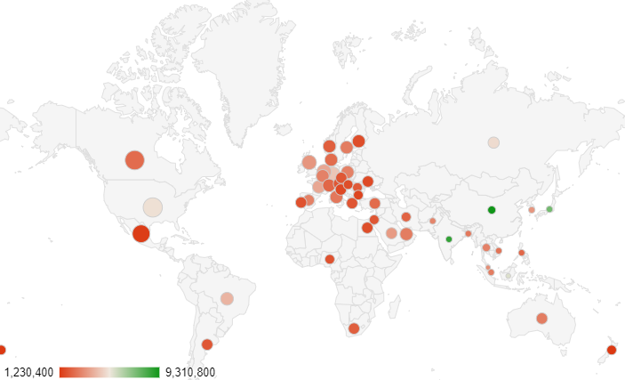
Google Sheets also allows you to create a Geo chart with markers, which is a bit similar but the difference is the countries are not filled in. Instead, there are circles representing the values.
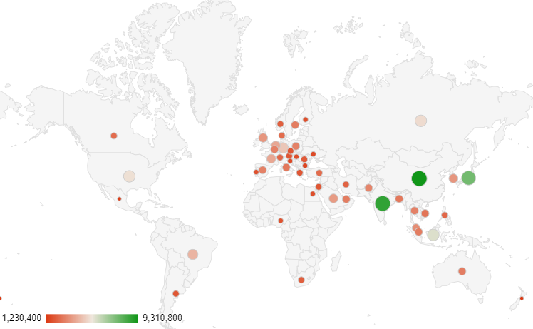
With this type of chart, you can add another field to track the size of the circles. In the following data table, I also have a field for the average sale price.
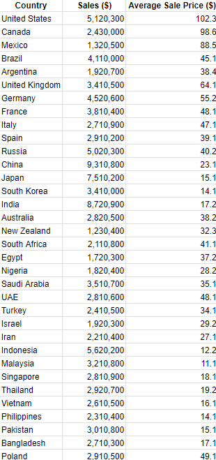
The average sale prices are highest in North America and smallest in Asia, and that is visually represented in the chart below. In addition to having the colors indicating the overall sales values, I can compare the average prices by looking at the size of the circles.
Overall, creating map charts is easy whether you’re making them in Excel or Google Sheets. In Google Sheets, however, there is some added flexibility, and the ability to use markers allows you to utilize an additional field in map charts.
If you like this post on Creating Map Charts in Excel and Google Sheets, please give this site a like on Facebook and also be sure to check out some of the many templates that we have available for download. You can also follow me on Twitter and YouTube. Also, please consider buying me a coffee if you find my website helpful and would like to support it.