goal seek inputs

Use Goal Seek to Avoid Trial and Error

Excel’s what-if-analysis options aren’t the greatest, but one option which is very useful and can save time is Goal Seek. What Goal Seek effectively does is it can do trial and error for you in seconds, and be much more precise than doing it manually.

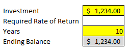
In many examples you could use algebra to get to your answer but if it’s a one-time calculation perhaps it’s not worth the trouble of going that route. For example, suppose I had an investment of $1,234 and wanted to know what average return would be needed for it to grow to $10,000 after 10 years. This can certainly be done with algebra, but Goal Seek can also do it. Below, I have entered my inputs in yellow.
goal seek inputs
My ending balance is equal to the following formula : =C4*(1+C5)^C6
C4 = Investment
C5 = Required Rate of Return
C6 = Years
Next, I will select Goal Seek from the Data tab under What-If Analysis

what if analysis
The next screen prompts me to enter which cell I want to set to which value, and which cell I want changed to accomplish this (the variable). In my example I use C7 for the set cell box (this is my desired ending balance), the value is 10,000, and by changing cell I enter my required rate of return (which is C5).
goal seek function
After clicking OK it fills in the required rate of return as 0.23273147. It also sets the value in C5 to this amount as well. If I hit OK on the next screen the value in C5 will keep this value, if I cancel, it will revert to what was there before – nothing.
goal seek analysis
This was a simple example but there are also more complex ones it can be used for. Another example could be an amortization table. The table below has a principal amount owing of 10,000, an interest rate of 5%, a payment of 550 per month. This is what it looks like:
goal seek amortization table

So it will take roughly 19 payments to for this amount to be paid off under the terms described. But let’s say I wanted to know precisely what interest rate would have to be applied to make the ending balance at payment number 20 equal 0. I don’t want an extra payment for the balance to be included at the end, just so that it perfectly matches 0 after payment 20.

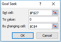
To do this, I go back to Goal Seek. For the first box (set cell) which is what I want my result to be – I select the ending balance at payment 20 – currently it is (579.34). This is cell F27 on my spreadsheet. The second box is what result I want, which in this case is 0. Lastly, my variable, or the cell I want changed to make this work – that is my interest rate, which is in cell C4 – currently it is at 5%. These are what my inputs look like:

goal seek interest rate

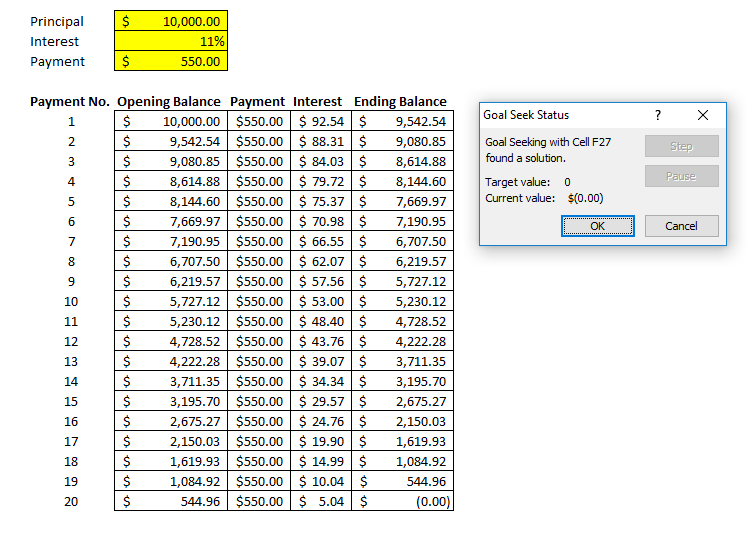
Once I hit OK, I get the following:
goal seek amortzation table
You’ll notice now my target value matches my current value and the Goal Seek was successful. It has changed my interest rate to 11% – not exactly 11%, 11.1048262490731%. A very precise percentage that has allowed my table to reach 0. 
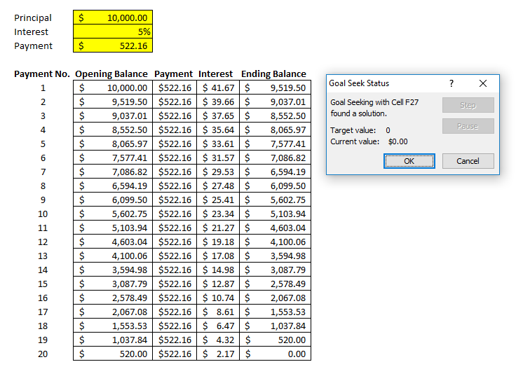
Goal Seek can be used in a variety of different circumstances as you can see. As long as you have a formula like in the above two cases that the change cell (e.g. variable) directly effects, then it should work. I could have selected the payment as my change cell rather than the interest rate and my result would be as follows:
goal seek amortization table
It would indicate a rounded payment of 522.16 (exact amount of 522.162995552194) would be needed to pay off after 20 payments with the interest rate staying at 5%.
The one limitation of Goal Seek is that you can only use one variable. But beyond that it does it very well and can help save you a lot of time.
aprogress

Show Progress Using a Picture in Excel

Please note this works only on versions of Excel 2010 and newer

There are many different ways to show progress in Excel, and in this post I am going to provide you a template to show you how you can do this through an image. Link to the template is here
In my example, I’ve inserted a picture of a glass of beer from clip art. In order for this to work I need two pictures of the same image. One that shows what the image looks like when at 100%, and one when it looks like when it is at 0%.
Certainly you don’t need to use clipart for this and can do it in a photo editing program but what I did was just used the picture editor to recolour the image with white, or ‘washout’
Now I have two images, I need to name the one that is empty as pictureempty, and the one that is 100% as picturefilled – this image needs to be on top of the pictureempty image. To do so you right click on the picturefilled image and select bring to front. Now, importantly, the images need to overlap one another. Carefully align the pictures so they are exactly overtop of one another. If they’re not, you’ll notice after running the macro anyway and can adjust accordingly.
Once you’ve got them aligned then all that’s left to do is change the percentage and click the update button and you will see the picture be filled from bottom to top based on the percentage you have entered in. Without clicking the button it will not update.
Inventory count sheet showing data by product number.

How to Sort Data in Excel Without Messing Up Formulas

If you have a formula that involves multiple sheets and you later sort that data you may notice your cell references are now out of order and need to be corrected. It can be frustrating and dangerous because you may not realize your formulas are now calculating different cells.

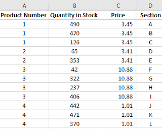
For example, I have created a sheet called InventoryCount and another called Total. The InventoryCount sheet acts as a tally of all the locations a certain product number is found:

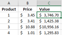
Inventory count sheet showing data by product number.

On the totals sheet, I have a summary of these product numbers using a SUMIF formula that multiplies by the price.

A summary of the inventory values.

The formula in the highlighted cell above is as follows:

=SUMIF(InventoryCount!A:A,Total!A2,InventoryCount!B:B)*B2

The formula in the price column for product 1 is:

=VLOOKUP(A2,InventoryCount!A:C,3,FALSE)

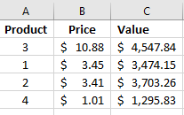
Both formulas are referencing the InventoryCount sheet. The formulas in the value column are correct. But let’s say that I want to sort that column by values. If I sort in descending order, this is what I get:

Inventory data after applying a sort.

The values are not only not correctly sorted  (product 1 is lower than product 2’s value) but the values have changed. If you look at the values before the sort product 3 dropped from 10,956.16 to 4,547.84. There is nothing glaringly obvious that the calculation is now completely incorrect so you can imagine the danger when dealing with lots of data that such a sort could make your data get altered. The formula for the value in product 1 now looks like this:

=SUMIF(InventoryCount!A:A,Total!A2,InventoryCount!B:B)*B3

It is still referencing A2. So technically the formula is still correct, the problem instead is product 1 is no longer on row 2, it is on row 3. The assumption that the value in row 3 relates to the product on row 3 will now be incorrect.

So why did this happen? Notice that the price has not changed for any of these products, Product 1 was $3.45 before the sort, as well as after. This column still is correct in relation to its corresponding products.

If you go back and look at the two formulas (price and value) you will notice on key difference: the cell referenced on the current sheet (Total) for the price does not mention the sheet name, however on the value formula it does.

This is the original formula to calculate the value:

=SUMIF(InventoryCount!A:A,Total!A2,InventoryCount!B:B)*B2

The Total! reference is causing the sorting issue and needs to be removed. The updated formula becomes:

=SUMIF(InventoryCount!A:A,A2,InventoryCount!B:B)*B2

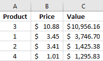
Now if I apply the same logic to the other formulas in the value calculation and sort the data in descending order, below is the result I get:

Inventory data after applying a sort.

The values are back to what they were at the start and product 3 is the highest as it was initially. Except now they are correctly sorted in descending order with the product number correctly being referenced in column A.

So the lesson here is that if you are using formulas with multiple sheets get rid of the sheet reference when referencing a cell on the same sheet as the formula is on (Excel inserts this reference automatically as you switch from one sheet to the next). Otherwise, if you or anyone else sorts the data the calculations will not be on the correct rows.


If you liked this post on How to Sort Data in Excel Without Messing Up Formulas, please give this site a like on Facebook and also be sure to check out some of the many templates that we have available for download. You can also follow us on Twitter and YouTube.

Ranks in Excel: Breaking Ties

The RANK() function in Excel is limited to a single range and if you do not have a set of unique numbers to use the rank function on it will return repeating values.
There is a workaround however. If you can afford an extra column for a ‘rank total’ then it will be easy to accommodate. Or you can use an array formula.
The easiest example in creating a rank total column is to look at standings in sports:
Team
W
Points
GF
GA
Goal Differential
Team A
5
15
20
5
15
Team B
4
12
19
18
1
Team C
6
12
12
7
5
Team D
4
11
17
15
2
In this scenario I’m going to say the rank order will first be by points, the first tiebreaker will be wins, followed by goal differential. My rank total formula will be as follows: Points + wins/100 + goal differential/10,000. I’ve broken out how the values look and after totaling them:
Team
W
Points
GF
GA
Goal Differential
Win Value
Differential Value
Rank Total
Team A
5
15
20
5
15
0.05
0.0015
15.0515
Team B
4
12
19
18
1
0.04
0.0001
12.0401
Team C
4
12
12
7
5
0.04
0.0005
12.0405
Team D
4
11
17
15
2
0.04
0.0002
11.0402
For Team A, their rank total is made up of 15 (points), .05 (wins) and .0015 for goal differential. If the factor for goal differential was only 1,000, then goal differential adds 0.015 and now it affects the decimal position for wins and has the same effect as a sixth win, which is wrong. So you want to choose your factors carefully so as not to effect the higher ranking tiebreaker. If goal differential was only ever single digits then you could have used a denominator of 1,000 instead of 10,000.
The result of this rank total tells me Team C should be ranked higher than Team B because both teams have the same points, same wins, but Team C has the higher goal differential.
Now what you can do to pull the ranks is use the following formula:
RANK(ranktotalvalue, ranktotalcolumn)
Or if you want to put the name of the teams in order of their rank rather than just saying Team A is in position 1, then you can use the index and match functions as follows. Assume the Team column is column A and the rank total is column I:
=INDEX(A:A, MATCH(LARGE(I:I,ROW(A1)),I:I,0))
Let’s break down this formula:
=INDEX(A:A
This tells the formula I want to extract the value from column A.
LARGE(I:I,ROW(A1))
This extracts the largest value in column I. The reason I use ROW(A1) instead of the number one is because now if I drag this formula down the relative reference will become ROW(A2), ROW(A3), and ROW(A4) which then looks for the second, third, and fourth largest values respectively.
MATCH(LARGE(I:I,ROW(A1)),I:I,0)
This formula looks for where the value matches the result of the large formula calculation. Where that match is made, the related value from column A is returned. And the following list is generated:
Team A
Team C
Team B
Team D
This correctly puts Team C ahead of Team B in the rankings.
WHAT IF I DON’T HAVE ANY TIEBREAKERS?

If you do not have any tiebreakers then what you can do is pull them in the order that they appear. If you want them to be in ascending or descending order, then you will first need to sort the data in such a way.
In this case, you can calculate your rank total using a value for the row the values are on. The formula for the ‘row value’ would be calculated as follows: 1/(ROW()*100).  The fraction is used to make sure the rows higher up will appear first. I multiple the denominator by 100 to push it further down the decimal location. Below is how my rank totals now look:
Team
W
Points
GF
GA
Goal Differential
Row Value
Rank Total
Team A
5
10
20
5
15
0.005
10.005
Team B
4
12
19
18
1
0.003333333
12.00333333
Team C
4
12
12
7
5
0.0025
12.0025
Team D
4
11
17
15
2
0.002
11.002
I changed Team A’s point total to 10 for the sake of this example. Now the top two ranked teams (B and C) both have 12 points. Because B is in a higher row and thus shows up before C, it has a higher row value which in turn gives it a higher total rank value. So the correct order now is Team B, Team C, Team D, and Team A.
THE FORMULA METHOD

Now if you don’t have the luxury to put an extra column in your worksheet, you can certainly do this in a formula, although it won’t be pretty. Essentially you’ll recalculate the rank total and search through the values using an array formula.
To recalculate the rank for the non-tiebreaker method:
{=INDEX($A$2:$A$5,MATCH(LARGE(($C$2:$C$5)+(1/(ROW($G$2:$G$5)*100)),ROW(A1)),$C$2:$C$5+(1/(ROW($G$2:$G$5)*100)),0),1)}
The INDEX formula again looks at the Team column while looking for the largest value when adding the points value to the row value. The calculation for the row value is the same as above just now dumped into a formula. An array formula has to be used to ensure each team’s results are looked at individually.
For the multiple tiebreaker scenario from above, the formula will be longer to accommodate for all the extra tiebreakers it has to look at:
{=INDEX($A$2:$A$5,MATCH(LARGE(($C$2:$C$5)+($B$2:$B$5/100)+($F$2:$F$5/10000),ROW(A1)),(($C$2:$C$5)+($B$2:$B$5/100)+($F$2:$F$5/10000)),0),1)}
Again, same logic and formulas are involved except without a rank total column it has to be done in an array. The results yield the same order as through adding an extra column.

Simple VBA Tricks

A couple quick snippets of VBA code that can help you impress your friends although might not have much real utility.

First up: have Excel speak to you

Application.speech.speak “text”

Where text is what you want Excel to say. Just like with any other code you can of course use variables for this to alternate. You could create a list to cycle through various messages as well.

Another one: opening a URL

ThisWorkbook.FollowHyperlink “http://www.google.com”

The above code will open Google when triggered in the default browser.

Removing Blank Spaces

When copying data into Excel from other sources – be it web pages, documents, or other Excel documents sometimes you end up with unwanted formatting, such as numbers with invisible spaces that prevents it as being read as a number or converted into one. Or just ending up with data you don’t want.
The TRIM function in Excel is useful for removing trailing spaces after text that serve no purpose.
The more annoying issue that I’ve come across is a blank space that looks like one but isn’t. It is usually character # 160 which looks just like a blank space, only thinner than normal. If you enter char(160) in a cell you’ll see what this looks like. It can be a frustrating process because this character you can’t get rid of by just searching for blank characters and doing a find and replace or the trim function. It’s possible to see this with other characters as 160 isn’t the only one that looks like a blank space, but it is the only one I’ve come across so far.
The solution is to replace character 160 with character 32 (this is a normal space that will get eliminated with the TRIM function). To do this, use the following formula, assuming cell a1 is the cell that needs the cleanup:
=TRIM(SUBSTITUTE (A1,CHAR(160),CHAR(32)))
You can add a *1 to the end of the formula to convert it to a number if necessary.
See below for an example. The only difference between the cells in A2 and A3 is A2 has a normal blank space after it whereas cell A3 has character 160 after it. Both cells equal the same length (12 characters) as show in column B. column C is what the cells look after using the TRIM function – they will look the same but column D recalculates the length and the top cell has now gone down by one character (the trailing space). Column E is after the above formula is used. You can see now the updated length in column F is 11 for both, meaning the trailing character has been deleted in both cells.

As a side note, if you’re need to reference a specific character in excel you’ll notice all it takes is using the CHAR formula. If you’re not sure which number of the character you need, you can have the CHAR function reference the numbers 1 to 255 and you’ll see all the different characters available.

Pivot Tables: Avoid Changing Data Sources with Named Ranges

When working with a pivot table, you determine a data source to use for that table. But what if later you add rows or columns? You’ll normally have to change the data source to include the updated range, otherwise your pivot table isn’t including your changes. Unless you use a named range.

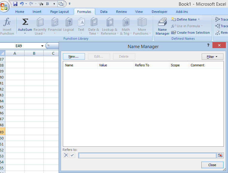
First, select the Name Manager under the Formulas tab and click on New

However, instead of selecting all the data, I’ll use the offset formula.

The OFFSET function allows you to specify the size of your data set. The formula below will keep the range equal to all the nonblank rows and cells starting from cell A1:

=OFFSET(Sheet1!$A$1,0,0,counta(Sheet1!$A:$A),counta(Sheet1!$1:$1))
This is the first cell of your data source

This is the first column of your data source

This is the first row of your data source

Once you’ve created a new name for your data set, put the formula above in the Refers to field and press OK:


Now you’ve created your custom, auto-updating range. All you need to do now is when creating a pivot table (or changing its data source), put in the named range.

Note this will not work properly if you have gaps in your columns or rows. The COUNTA function counts how many non-blank cells are within the range. So you could manually override the formulas if need be, but that would defeat the point of this post.

But if you follow the above steps and use the formula above, your pivot table will automatically be updated with any new rows or columns you add to it. All you’ll have to do is refresh the pivot table. And because the offset formula forces the range to change, that will automatically happen in the pivot table as well.

Highlight Alternating Rows or Columns

This post will show you how to create the effect of highlighting alternating rows, which sometimes makes it easier to read a data set.

In order to accomplish this, first select all the cells in the worksheet and then select New Rule under conditional formatting.

For the new rule you will need to select the last option to use a formula. The formula we will need to use is as follows:
=MOD(ROW(A1),2)=1
The MOD function calculates the remainder after division and has two arguments, the number to be divided into, and by what number. 
Using ROW(A1) means the reference will change depending on the location of the cell, meaning it will encompass every row in the selection. Using 2 as the divisor will help identify if the row is as odd number or even. If you’d rather highlight columns than rows, use the COLUMN function.
The formula will be true if the remainder is 1, meaning the row is an odd number (e.g. highlighting will start on the first row). If you want highlighting to start from row 2, just change the 1 to a 0, since even rows will have no remainder.
Once the formula is set, click on Format to determine the appearance of the alternating rows.
I select a light blue colour for the alternating rows
After I press OK this is the result of my conditional formatting:
If you don’t want to apply the formatting to all the cells or want to change the range, under conditional formatting select manage rules
There you will see a field where the formatting Applies to. Here you can change the range you want the formatting to apply to.