conditional formatting – Page 2

Color Calculator Template: Sum by Color in Excel

July 11, 2020

by howtoexcel with No Comment conditional formatting formatting template

Unless you’re still stuck on old versions of Excel, you probably know that you can filter data using colors. And by doing so you can use the SUBTOTAL function in excel to tabulate those amounts. But in this post, I’m going to show you something a little different. By using a macro, I’ll highlight cells containing values and then sum them by color in Excel, without needing a subtotal or a filter. This free template will just use VBA to populate the totals.

How the template works

In this template, all you need to do is enter your data and then assign whatever formatting you want to use to identify a cell to the corresponding category. As long as a cell has the exact same formatting as the category, it will be included in that category’s calculation.

I got the idea when I was trying to quickly analyze expenses and didn’t want to go through a whole process of putting it into a complex budget template. Rather than setting up logic to classify whether an expense falls into one category or another, I thought color-coding could be another way you could quickly group expenses.

Here’s a quick video showing you the template in action from color-coding cells to calculating the totals:

Setting up the data

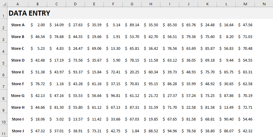
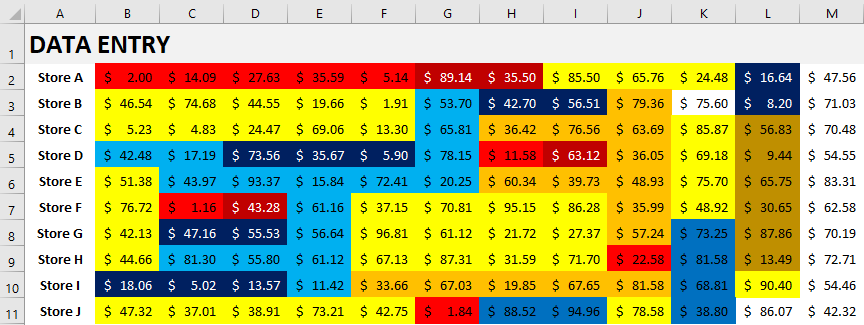
In the template, there’s one section dedicated to the raw data where you’ll enter your inputs:

You can input data up until column N, although I’ve left the column blank for a buffer. In this example, I’ve put in random numbers and grouped them based on a store value in column A. This can be all numbers, it doesn’t really matter, I just preferred to have some grouping.

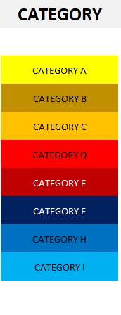
Next to the data entry, I’ve got a list of categories set up in column O:

You can add as many categories as you like. How they’re color-coded here is how you’ll need your cells will need to look to ensure they’re in the correct categories. For instance, any cells that are highlighted in light blue will go into Category I. Whereas anything in a dark red will belong to Category E.

You may think this would be a painful process to try and color-code your data based on all these different categories. After all, what if you get the shade wrong or the font color is wrong. The solution’s really simple and you just need to use our trusty friend, the Format Painter. If you’re not familiar with it, this is what it looks like:

It’s on the left-hand-side of the Home tab where the copy buttons are. What you can do is select the category you want to be assigning data to, click once on the Format Painter and then click on the cell you want to highlight with that exact same formatting.

If you’ve got multiple cells that you want to apply the formatting to and don’t want to keep repeating this exercise, then Double-Click on the Format Painter. You can now continue selecting cells and the Format Painter will take care of the formatting for you. You won’t need to re-select it each time. Once you’re done with the formatting and want to stop applying it, click on the Format Painter again to stop.

I’ve color-coded some of my data based on the categories, and here’s how it looks:

Updating the calculations

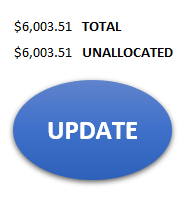
On the right-hand-side of the page there’s a button that says Update. This will update the totals based on the color-coding. You’ll need to have macros enabled for this to work. Above the button you’ll see the total of all the values in columns and how much is unallocated.

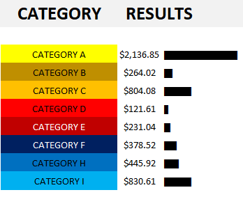
Clicking on the update button will trigger the macro to run the calculations. After pressing the button, here’s what my categories look like and the totals corresponding to their color-coding:

You’ll notice I’ve also created visuals to see the relative size of each category using the REPT function. If you’re interested in learning how to use this function, check out this post.

Anytime you make changes to the color-coding, be sure to hit the Update button. I didn’t want the formulas to update every time there was a change on the sheet because that can sometimes slow a spreadsheet down, especially since it would involve recalculating all the totals.

The code

Here’s the VBA code itself on how the update button works:

Sub Oval1_Click()

Dim clvalue, clcolor As Double
Dim cl, colorrange As Range
Dim lstrow As Integer

lstrow = ActiveCell.SpecialCells(xlLastCell).Row

Set colorrange = Range("colorrange")

'clear data range
colorrange.Offset(0, 1).ClearContents


For Each cl In ActiveSheet.Range("A1:O" & lstrow)

    If IsNumeric(cl) Then
    
        clcolor = cl.Interior.Color
        
            For Each lookupcl In colorrange
    
                If lookupcl.Interior.Color = clcolor Then
                    lookupcl.Offset(0, 1) = lookupcl.Offset(0, 1) + cl.Value
                    GoTo nextcl:
                End If
    
            Next lookupcl
    End If

nextcl:

Next cl

End Sub

There’s a named range called “colorrange” that it cycles through, and those are the categories in column O on the spreadsheet.

Using the template

This isn’t a terribly complex template to use. However, it can help if you want to quickly group items. It’s a unique way to classify expenses rather than just using drop-downs and complicated formulas. And it makes it easy to sum data by color in excel. The way I found it useful was to list your vendors or stores in column A. Then, arrange transactions by date (e.g. the first transaction is in column B, then C, and so on). But this can be used in a variety of different purposes to help classify data.

If you want to reset the calculations, just change the data back to the default formatting or something that doesn’t correspond to a category you already have, and then click update.

Download

The template is free to download and it’s available here.

If you liked this post on how to sum by color in Excel, please give this site a like on Facebook and also be sure to check out some of the many templates that we have available for download. You can also follow us on Twitter and YouTube.

How to Hide Zero Values in Excel

February 1, 2020

by howtoexcel with No Comment conditional formatting errors formatting iferror intermediate tips & tricks

If you’ve got a big spreadsheet with lots of numbers to look at, it can sometimes be a bit difficult to look at a large chunk of data. That’s where knowing how to hide zero values in Excel can be helpful in reading and analyzing data in Excel. By not seeing the zero values, you can easily focus your eyes on the more important numbers that may need more analysis.

However, it doesn’t have to be just zero values that you hide. Any number that’s insignificant for your analysis can also be hidden. For instance, you can be analyzing a company’s financial performance and choose to hide any movements that are less than 5%. The same principles apply as you would use to hiding zero values. Below, I’ll show you how you can hide not just zero values but any values that you don’t want showing up in your data while still factoring them into totals and any other calculations. You won’t be deleting anything, just masking the information.

First, let’s take a look at how to hide a potentially even bigger nuisance: errors.

How to hide errors on a spreadsheet

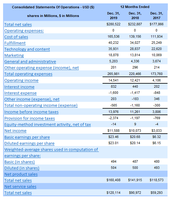
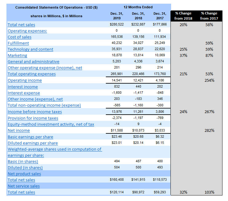
To help illustrate how to hide zeo values in Excel as well as other numbers, I’m going to use some real-world data — Amazon’s most recent annual earnings report, which the company released last month. Here’s the company’s income statement from the past three years:

Amazon's income statement over the past three years in Excel format.

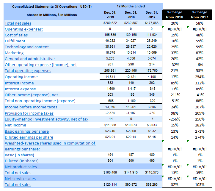
If you’d like to follow along, you can download the data from the SEC. First up, I’ll add a few columns showing the change from 2018 to 2019 and from 2017 to 2019. Here’s how it looks just copying the formulas straight down:

Analyzing Amazon's income statement using Excel with error values showing.

I have divide by zero errors as there are rows that have no data. I could just remove these cells but as with anything in Excel, it’s good to be consistent. Rather than deleting those error values, I can get rid of the errors in one of two ways.

The first is by using an IF statement to say that if the denominator is 0 or blank, to ignore the calculation. The second is just to use an IFERROR statement.

Here’s what my formula looks like for the 2018 to 2019 change:

=C5/D5-1

Where C5 is the 2019 data and D5 the 2018 numbers. I don’t need any parenthesis as order of operations ensures the formula will calculate properly. However, it doesn’t prevent me from getting a divide by zero error. Since the numerator can be blank or zero, what I’ll want to focus on is fixing the denominator in D5. To do this, I can add an IF function that looks at whether the denominator is a number. Here’s what my formula will need to look like to remove that error:

=IF(OR(D5=0,D5=””),””,C5/D5-1)

The formula now checks to see whether D5 is either a zero or blank, and if it is, it returns a blank value. Otherwise, it calculates as normal. Now I can copy this formula down and get rid of the error values.

An alternative way to fix this is by using IFERROR. Introduced in Excel 2007, the function can be an easy way to replace errors on your spreadsheet with another value. In this example, I’m going to use empty quotes (“”). The benefit is obvious: it’s a lot easier to use IFERROR than an IF statement, especially combined with an OR function as well. Here’s what my formula would look like with IFERROR:

=IFERROR(C5/D5-1,””)

It’s a whole lot easier and quicker. I don’t have to worry about the logic and all the reasons why the formula might error out. However, it’s not a perfect solution and here’s why: it will correct errors, but it’s possible they’ll be errors you’re not expecting. For instance, if I copied the data wrong or keyed something over and put text in a field where it should be a number, the IFERROR will correct that and you won’t be able to tell whether it’s blank because it is a divide by error problem or something else. That’s where it can be a little dangerous in using this one-size-fits-all approach to fixing error values. As long as you’re okay with that, it’s a perfectly good approach to fixing the divide by zero errors.

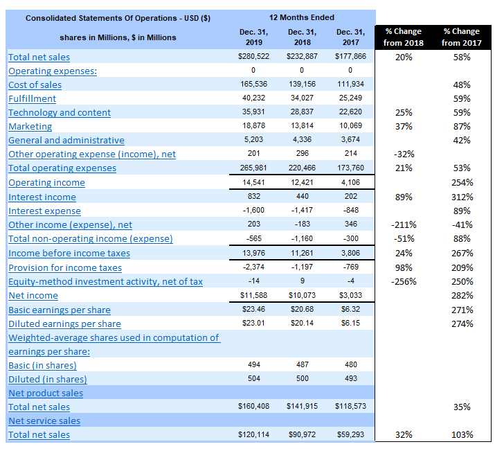
Here’s the data now that it’s been cleared of errors:

Analyzing Amazon's income statement using Excel after error values have been hidden.

That looks a lot better but the problem is that it’s still a lot of percentages to look at and it’s difficult at a glance to see what are the big changes are from the prior year. This is where it’s also important to hide zero values in Excel, as well as low values that aren’t useful for analysis.

How to hide zero values in Excel and other numbers that you don’t want or need to see

In order to hide data, it’s useful to use conditional formatting. If you’re not familiar with how to use conditional formatting, check out this post. Conditional formatting won’t remove or erase any data, which makes it a good solution that will keep all the data and calculations intact.

In the Amazon example, there are some pretty large-moving items in the list. Removing zero values won’t do anything and the threshold needs to be big for it to be helpful in hiding the lower values. Let’s start by removing the percentages that are less than 20%. Here’s the formula that I will use in the conditional formatting to accomplish this:

=AND(F5<0.2,F5>-0.2)

Column F is where the % Change from 2018 values are. I need to use the AND function because if I just look at anything that’s less than 20% this will also capture negative movements that are more than 20%. And for now, I want to keep those. I want to remove anything that’s between -20% and +20%, which is what the above formula will capture. If I was only looking to remove the zero values then the formula would be as simple as F5=0.

The next step is to adjust the formatting so that the cell font is white. Changing the color is an easy way to hide a cell’s value if it’s on a white background. While that data is still there, it won’t be visible:

Analyzing Amazon's income statement using Excel with error values fixed and low values hidden.

It creates a lot more white space, allowing me to see a lot more of the bigger values. The problem that I notice, however, is that there are some low values that are creating big movements in percentage. I can go a step further and create another conditional formatting rule that will also ignore the percent change for any item in 2019 that was less than $1 billion (1,000). This is how that formula will look:

=$C5<1000

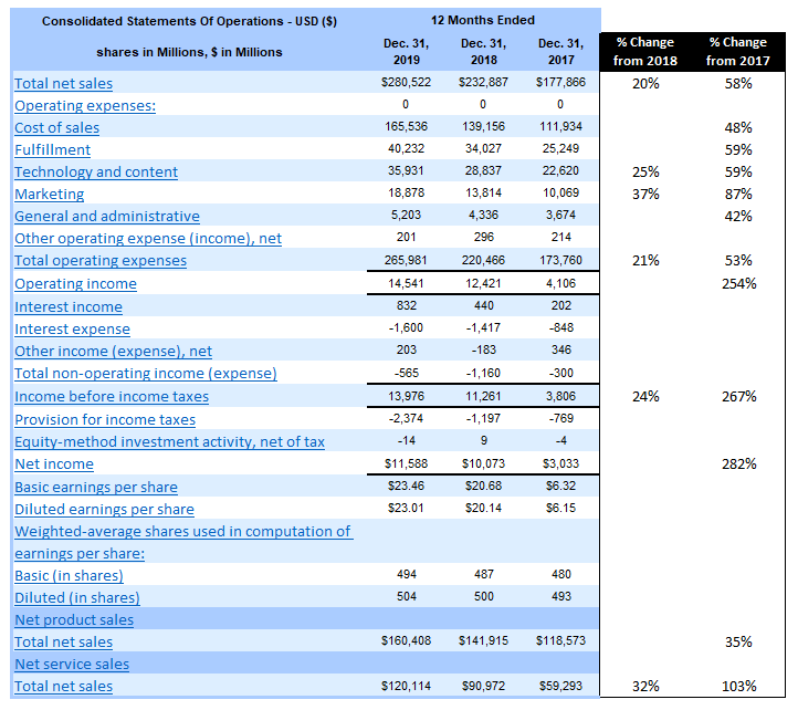
I need to freeze column C because the conditional formatting will be used for the other change column as well and I don’t want the reference to move. Now, with this adjustment, it makes a much bigger difference and helps me narrow in on fewer items:

I can see that the significant changes from 2018, besides the totals, were in sales, technology and content, and marketing. However, since the growth rate from 2017 is even higher, I’ll need to adjust those percentages to also ignore anything that’s not at least a 50% improvement. Here’s how that formula will look (note that I’ll only apply it for the % Change from 2017 column):

=AND(G5>-0.5,G5<0.5)

Remember, since I’m analyzing percentages, these figures need to be in decimal point. Otherwise, I would be using whole numbers. With those changes, this is how my data looks:

Now I’ve also got a reasonable amount of items I can focus on for the % Change from 2017 column. In addition to the same items increasing from 2018, I notice that fulfillment costs have also shown a significant increase over two years.

The conditional formatting works great in clearing out numbers that I don’t want to see. However, there’s just one small problem…

Analyzing Amazon's income statement using Excel with hidden values showing on a dark background.

If I change the color to anything that isn’t white, those numbers that I hid become visible again. That leads me to another all-important section:

How to hide values in Excel that are on different background colors

You can create conditional formatting rules to address other background colors but that’s just not practical. If you use lots of colors on your spreadsheet the last thing you want to do is create a rule for every different color and make sure the cells are hidden in the same font color. There’s also a problem if someone changes the color too.

That’s why using font color to hide values in Excel isn’t a good idea. The good news is that there’s a much easier way to hide values that doesn’t involve you having to try and match up the color.

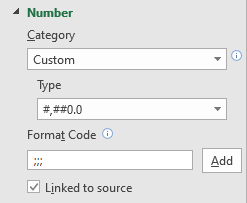
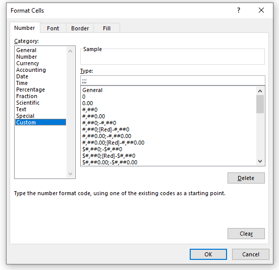
Rather than changing the color, what you should do is use a custom number format. Simply use three semi-colons and that will do the trick:

Choosing a customer number format to hide zero values in Excel.

Without going into the details of the different formats you can use, by using three semi-colons you’re telling Excel that you want no formatting to be used whether the amount is positive or negative. Now, my hidden data remains hidden regardless of the background color:

Analyzing Amazon's income statement using Excel with hidden values no longer showing on a dark background.

Now you don’t have to worry about background colors and can easily hide your data in any context.

If you liked this post on how to hide zero values in Excel as well as other values, please give this site a like on Facebook and also be sure to check out some of the many templates that we have available for download. You can also follow us on Twitter and YouTube.

How to Alternate Row Color in Excel

November 28, 2019

by howtoexcel with No Comment conditional formatting formatting functions intermediate

Looking at numbers on a plain white spreadsheet can sometimes make it difficult to differentiate one row from another, especially from afar. It can also make the spreadsheet look a bit bland. That’s why in this post I’ll show you how in Excel you can alternate the color of both rows and columns.

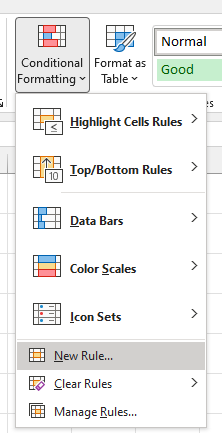
The first step is to create a new conditional formatting rule in Excel

Ultimately, all you need to alternate the row color in an Excel spreadsheet is a little bit of conditional formatting. It just comes down to getting the logic and the formula right in ensuring that the correct rows are highlighted.

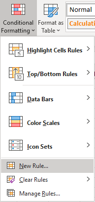
To get things started, select Conditional Formatting from the Home Tab and then Create New Rule

home tab excel selecting new rule from conditional formatting menu

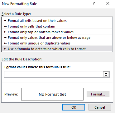
Once there, you’ll want to select the option to Use a formula to determine which cells to format:

selecting a formula for conditional formatting in excel

This is where we’ll now enter the formula that we’ll want to use for the alternating rows.

Use the MOD function along with ROW to determine which row to apply a different color to

The key function that we’ll need to use is the MOD function. What this function does is it tells us what the remainder is after a number has been divided by a divisor. This is important because what we need the conditional formatting to do is to evaluate each individual row to tell us whether it is an odd or even number, and the MOD function allows us to do that.

For example, the following formula will return a value of 0:

=MOD(6,2)

Since two divided by six will return a result of three and have no remainder, the result of the formula is 0. If, however, we change the formula to this:

=MOD(6,4)

The formula will now return a value of two, since four only goes into six one time, leaving a remainder of two.

Now, it’s simply a matter of applying this logic to each row. To do this, we need to incorporate the ROW function into our formula as well. The end formula is actually not very complex:

=MOD(ROW(),2)=0

The above formula will be true if the row is an even number, and thus, any conditional formatting we have set for that rule will apply. If we wanted to modify every odd row, then the formula could be tweaked as follows:

=MOD(ROW(),2)=1

You could have two sets of rules, one for odd rows and one for evens, but that’s really not necessary. Instead, you can simply select all the rows and then apply the formatting you want for the even rows, and then create a conditional formatting rule for the odd rows. This way, the formatting you apply to the entire sheet will be overwritten by the conditional formatting rules for the odd rows anyway and your original formatting will end up applying only to the even ones.

Applying a different color to the different rows

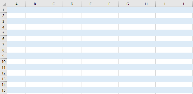
Once you’ve created your rule, then it’s just a matter of selecting the formatting you want to use and how you want to highlight the rows. I’d suggest a color that is light so that you don’t have too much contrast. This is how my Excel spreadsheet looks after applying a light blue color to every alternate row. I’ve left the default formatting in place for the odd rows.

conditional formatting alternating rows highlighted

If your spreadsheet doesn’t look like this, check to make sure that you have applied the conditional formatting to the entire sheet and that it isn’t only to a select few rows or cells. If you’re unsure about this, refer back to my earlier post on conditional formatting to help give you a better idea of how it works.

You can highlight alternate columns in a different color too

As you may have guessed, the same logic and conditional formatting rules that we used above can be applied to columns as well. Instead of the ROW function we just need to use the COLUMN function in our formula. That’s really the only difference as the formula will look nearly identical:

=MOD(COLUMN(),2)=1

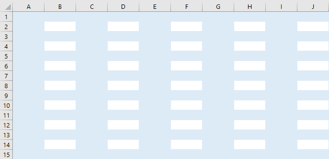
You’ll follow the same steps as far as creating a new conditional formatting rule, but the process is largely the same. The one thing that you’ll notice, however, is that if you have both rules in place, your conditional formatting has now overlapped:

conditional formatting overlap for both columns and rows in blue

In the above example, the formatting is the same color, but if they were different, the overlap would stand out even more. And that’s where it may take some experimenting with different formats to ensure that you get the right overlap and that the different formatting rules blend well together. Assuming, of course, that you want both rules in place.

Other options to alternate the row and column color in Excel

While this post showed you how to change colors for odd and even rows and columns, you can certainly extend that logic even further. For instance, you could decide to highlight every third row by changing the MOD function so that you’re dividing by three rather than two. As long as the logic is sound, you can modify these formulas so that they alternate the rows that you want.

For example, if you wanted to alternate the color of every fifth row and every 13th row on your Excel spreadsheet, you could create one conditional formatting rule to apply to every fifth row and then another for every 13th one as well. Although putting this into one larger formula is possible, it would a bit cleaner to put them into different rules.

When it comes to conditional formatting, there’s a lot of flexibility in how you can structure how your spreadsheet works. However, you also don’t want to get too carried away and make the spreadsheet too colorful and difficult to read. Otherwise, it may end up defeating the purpose and making your spreadsheet less user-friendly.

If you liked this post on How to Alternate Row Color in Excel, please give this site a like on Facebook and also be sure to check out some of the many templates that we have available for download. You can also follow us on Twitter and YouTube.

How to Apply Conditional Formatting to a Bar Chart

September 14, 2019

by howtoexcel with No Comment charts conditional formatting intermediate tips & tricks

When using charts, sometimes you’ll want to highlight items differently depending on if they’re positive or negative, or may if they’re above or below a benchmark or average. While you can apply conditional formatting to cells, it’s not as easily done if you want to do the same to a bar chart. There’s no simple way without it involving a manual process. However, the good news is there is a workaround.

I’m going to use data from my 12 most recent stock picks on fool.ca and how they’ve done over the course of the month they were picked:

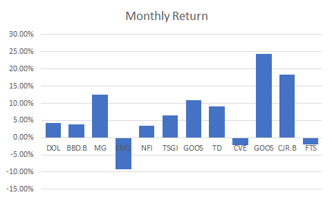
If I were to map the above table out in a bar graph, here’s how it would look:

Adding a column to add another series you can format

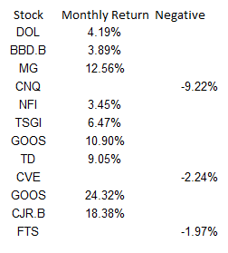
While the above chart is a good way to illustrate the performance, if I want to adjust the values so that they’re negative if they’re red, what I’ll want to do is add an extra column:

Then it’s just a matter of updating the chart so that the extra column is included, and changing the color of all the items on the negative series to red. This is also where you can apply whatever formatting you want to the specific series, and hence, conditionally format the results:

monthly returns table bar chart negative

Make sure you’re using a stacked chart

The one thing that looks off in the above chart is that the red numbers are on the right-hand side and the blue (positive) numbers are off to the left. To fix this, I’m gonna the chart type to a stacked chart. Then my chart looks like this:

That looks a bit better and is more what I was hoping to achieve.

However, I can even take this a bit further and add more columns. As long as it’s in a stacked chart and only one number is filled in for a column, you can have a lot more customization.

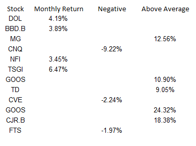
Adding a column for above-average results to add more conditional formatting

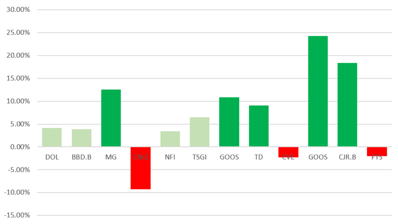
What I can do to help further differentiate the results is to create a column for above-average returns. To do this, I’ll add another column. I could do an if calculation to see if the number was greater than the average of 6.65%. You can have as many columns as you need to help get the number of groups you need. For example, you might have one column for the return, then a separate column for each group that you want to classify the numbers in. In this example, I just used three columns:

Note that what’s key here is that an amount only shows up in one of the three columns. If there’s any overlap, you’ll have multiple colors per item and then that will defeat the purpose of having only one color.

Below is what the chart looks like now, with bright green showing above average, red being negative, and anything else being light green:

monthly returns negative bar chart average

Although conditional formatting isn’t very intuitive when it comes to a bar chart, there are ways around it that you can make it work.

If you liked this post on How to Apply Conditional Formatting to a Bar Chart, please give this site a like on Facebook and also be sure to check out some of the many templates that we have available for download. You can also follow us on Twitter and YouTube.

Paying Off Debt vs Adding to Savings: Analysis in Excel

September 9, 2019

by howtoexcel with No Comment conditional formatting financial analysis

Excel is a great tool for financial questions and analysis, and one popular one is whether someone is better off paying down their debt vs adding to their savings. There are temptations to both, but this is where Excel can help identify a clear winner.

As much as it is a math question, it’s also a question about opportunity cost. If you’re paying down debt then you’ll incur fewer interest charges, and if you add to your savings then you can earn more in interest income. While both options will put someone in a better financial position, that doesn’t mean that one option isn’t better than the other.

Adding to Savings

Typically, banks pay interest rates of around 1% at best, unless there’s a promotional period. But generally, you aren’t making much when it comes to your savings. However, if you’ve got an amount of $5,000 to add to your savings, then that will produce an extra $50 per year at a 1% interest rate, or about $4.17 per month. It’s by no means huge, but it’s still incremental income that can help grow your savings over time.

Paying down debt

If you’ve got credit card debt, however, you’re probably paying anywhere from 15% to 20% in interest. There are exceptions, but most credit cards will likely fall within that range. On a credit card with an interest rate of 20%, that’s going to be an annual interest charge of $1,000 on a $5,000 balance. And so by paying down off a card at that rate, you’ll be saving a lot in expenses.

Difference in interest rates is key

It’s pretty clear that it all comes down to the difference in interest rates, and that’s why paying down debt will always provide you with more of a benefit than adding extra cash to your savings will. While it might be tempting to add to your savings, the reality is that you’ll likely be losing in the long run.

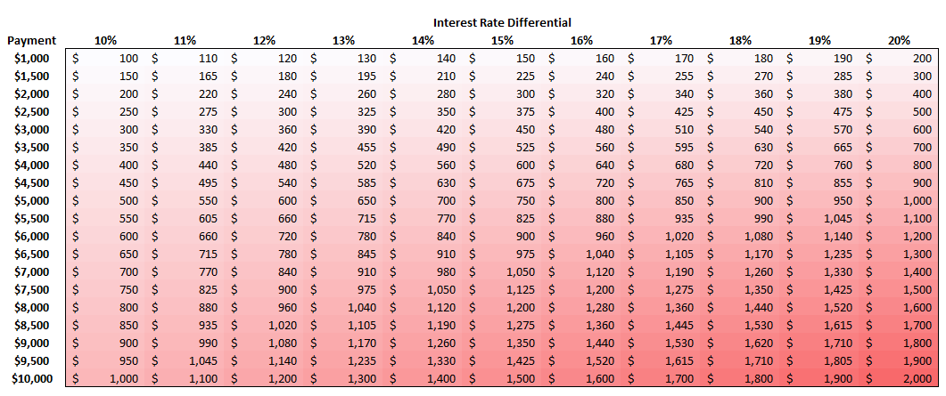
Using a color scale in Excel, I mapped out the difference in interest rates by the size of the possible payment. It’s a very linear relationship: the higher the differential and the higher the payment, the more money you’ll lose by putting money into savings rather than paying off debt:

In the example above, the difference in interest rates was 19% (20% in credit card rate less the 1% in savings rate). Multiplied by a $5,000 payment, that would have resulted in an annual loss of $950. Rather than avoiding $1,000 in interest charges, I would have made just $50 in interest income ($1,000 – $50 = $950 opportunity cost). On the matrix above, you’ll notice this is also the amount that is at the intersection of 19% and $5,000.

Summary

This isn’t the most groundbreaking discovery but it’s one that can be visualized well using Excel. After all, this is a numbers problem, nothing else. While some people may argue there are other reasons to add to savings such as having cash for a rainy day, the reality is that whether you add to your savings or free up room on your credit card, you can access funds from either option. And in the meantime, if you add to savings, you’re still incurring the interest charges. To make matters worse, the interest income you earn may be subject to income taxes, which will further erode the benefit of adding money to savings. Interest expenses on credit cards likely won’t be tax-deductible.

Overall, there really isn’t a strong argument for contributing to savings instead of paying down debt. It’s comes down to what interest rate you’re paying vs what rate you’re earning. And I’ve yet to see anyone earn more in interest than they’ve had to pay on a credit card.

The post is not a substitute for financial advice and is only intended to show how an analysis in Excel can be done when comparing two different options – in this case, paying down debt vs contributing to savings.

You can download the file that I used in these calculations here.

If you liked this analysis on Paying Off Debt vs Adding to Savings, please give this site a like on Facebook and also be sure to check out some of the many templates that we have available for download. You can also follow us on Twitter and YouTube.

Monthly Goal Tracker Template in Excel

August 1, 2019

by howtoexcel with One Comment calendar conditional formatting template

Whether you’re trying to lose weight or wanting to learn a new skill, sometimes it can be challenging to stay on top of those goals. One way to you can make that easier with this goal tracker template. It’ll allow you to keep a record of how you’ve done versus your goals and show you the progress you’ve been making. Just being able to see that progress can sometimes help encourage you to keep working at it, and this template will do just that.

The spreadsheet has two tabs: the calendar where you can select the month and year, and the data entry tab where you’ll enter your progress. Let’s start with the data entry since that is going to be where you make any changes and will serve as a starting point.

Setting Up Your Goals and Entering the Data

On the DATA.ENTRY tab, the first three rows are dedicated to the name of your goal, the frequency of it, and your desired target. The goal name is straightforward and doesn’t impact anything but what you’ll refer to it going forward. This can be changed at any point.

The second row is the frequency, and here you can enter either Weekly, Monthy or Daily. They’ll track your totals accordingly and which frequency you select will determine how the calendar will highlight your progress. As soon as you hit a goal that’s set to monthly, the spreadsheet will highlight the entire month in green to indicate that the goal has been met:

If it’s a weekly target, then only the week the goal was met will be highlighted:

Daily targets will only be highlighted one day at a time.

The third row on the data entry tab relates to the actual goal number itself. In my example, I’ve put 500 for the weekly amount of calories burned and 100 studying hours in a month. These are the metrics that will be tracked. They will reset each period as well so if 400 calories were burned in a week, that week won’t highlight in green. But if on the following week 500 are burned, then it will highlight that week.

For daily goals, no goal amount needs to be entered. You’ve either met the goal or not for that day, and avoiding numerical totals here will allow you just to mark an ‘X’ on whether you were on track for that day. This can be useful if it relates to a task that might not have a numerical value. It’ll also allow you to create a chain of X’s like the method made popular by Jerry Seinfeld.

goal tracker template excel daily x jerry seinfeld

This way, you’re not limited to trying to assign a number to every goal. If you do have a numerical goal for every day, you can simply convert that into a weekly or monthly total. The only impact there will be when the cells will be highlighted.

There’s no limit to the number of goals that you can have so you can have a mix of monthly, weekly and daily goals to suit your needs.

For the actual data entry itself, I’ve pre-populated a date of July 28 but you can certainly change that to a different start date. The data entry tab will auto-populate the next 365 days for you. However, you can certainly extend beyond that as well.

Once you’ve got your start date, you can start entering in your data. Just look for the date and goal name (top row) to make sure you’re entering it in the correct cell. For daily goals, simply mark an ‘X’ to indicate they were met. For weekly and monthly targets, enter a number.

The Goal Tracker Calendar

Once you’ve got your goals set up and your data entered, you can switch over to the GOAL.CALENDAR tab. Here, you can change the month and year that you want to look at, and select the goal as well, from the yellow drop-down directly above the date.

Once you’ve selected the goal, it’ll highlight whatever progress you’ve made. For daily goals, it’ll show any X’s, which will automatically be highlighted in green. For other frequencies, you’ll see the actual numbers themselves so you’ll see how you’ve done on each day.

You’ll notice that the calendar for August won’t start on August 1 but on the first day of that week. The purpose of this is to track those weekly goals as otherwise part of the week will be cut off and could appear like a goal wasn’t reached.

You can download the template here.

If you like this Monthly Goal Tracker Template, please give this site a like on Facebook and also be sure to check out some of the many templates that we have available for download. You can also follow us on Twitter and YouTube.

How to Make a Bar Graph in Excel Using a Formula

July 20, 2019

by howtoexcel with No Comment charts conditional formatting intermediate

Excel has a lot of charts and graphs that you can use to visually show data. However, there’s a way to create a graph using just a simple formula and applying some formatting to it. Below, I’ll show you how to make a bar graph easily without having to worry about legends, axis, or any other chart element you might otherwise need to manipulate.

The key function that makes this all possible is REPT, which just repeats a character a set amount of times. Here’s how it works in practice:

In the first argument, I specify the character that I want to be repeated. The | symbol, in this case, is repeated five times, which is what the second argument specifies. Right now, this doesn’t look anything like a bar chart, but that’s as easy as changing the font. Here’s how it looks like if the font is set to Britannic Bold and size 11:

If I had several of these values, I could make it look like a bar chart pretty quickly. Below are some random numbers from 1-10 and how I turned them into a bar chart using the earlier formula:

In the above formulas, I replaced the second argument with the numbers specified above. If an item had the number 10, the | character would be repeated 10 times.

Scaling the bar graph

Now, if you’re dealing with really small or really large numbers, your bar graph could look very skewed. What I’d suggest doing is determining how big you want your graph to look. For a column with a width of 15, I found that 35 characters would fill the bar chart all the way to the end of the cell (using the font type, size and character that I used above).

So to help make sure that my data was properly scaled, I’d calculate the maximum number from my data set, divide the specified number by that, and then multiply it by 35.

Here’s another example with numbers between 100-1,000, if I were not to adjust anything from the previous formula:

If I were to use the above formula as is, you can see my bar chart is going to explode with bigger numbers. So what I’d want to do is adjust the number of times the characters above repeat, to a maximum of 35.

First, I need to determine what value should maximize the cell or bar chart. In the above data set, 988 is the largest number. However, if my scale goes up to 1,000, that might be a better number to use as the maximum.

In that case, my formula for the number of repeats will look something like this: (value/1000)*35. That way, for the value 988, that will return 34.58 as the number of times I’ll repeat the | character. If I use that formula for the data, here’s how it looks now:

Adding more formatting

Now, I’ve got a bar chart that looks a lot more contained. However, this is still kind of a bit boring. So what I can do is add some conditional formatting to help make some of the items stand out a bit more:

rept function excel bar chart graph conditional formatting

In the above example, I set rules for anything below 300 to be highlighted red and anything above 800 to be green. When applying the conditional formatting, make sure you’re changing the font color, not the fill color. For more information on how to set up conditional formatting, check out this post.

If you liked this post on How to Make a Bar Graph in Excel Using a Formula, please give this site a like on Facebook and also be sure to check out some of the many templates that we have available for download. You can also follow us on Twitter and YouTube.

How to Setup Conditional Formatting (including Formulas)

June 7, 2017

by admin with 5 Comments conditional formatting formatting intermediate

Conditional formatting is useful for highlighting cells or ranges if a condition is true. For example: highlighting negative values as red or positive ones as green. You can also do more complex formatting like highlighting an entire row if it meets a criteria.

Creating A New Rule

To get started with conditional formatting, you need to select new rule from the conditional formatting options which is under the Home tab:

You will then have quite a few options as to what you want to do:

conditional formatting all cells based on values

Format All Cells Based On Their Values

This is useful if you want to show some sort of progression from one value to the next, as one colour will fade into the next. Here is an example using this conditional formatting on a range of values from 1 to 5:

1 started from the dark orange and gradually got to a light yellow colour by the time it got to the number 5. You can change the colours involved or even the range. You also can change the values instead of using lowest to highest values you can hardcode figures, use percentages, or whatever else. In all likelihood it will show something very similar regardless what you select, so leaving it to the default setting here (low to max) is going to be sufficient in most situations.

Another way you could use this formatting is if you wanted to compare a time-series. Assume the below are sales numbers and you wanted to highlight good and bad years.

You can see in this example there is no longer the smooth transition as in the prior example since I’ve assumed sales are bouncing up and down. The downside of using this type of conditional formatting as you could have a really colourful dataset if you did this.

You may like it initially but if you are dealing with lots of data it may not be all that helpful because you are dealing with many different shades of colours now and you may find yourself comparing different shades to see if one is darker than the next. And conditional formatting is most useful when you don’t have to spend time analyzing colours, and instead the colours help you do the analysis by easily standing out and highlighting what you want to see.

Format Only Cells That Contain

The next option on the formatting rules allows you to specifically look at the cell values. Keeping my sales numbers example from above I want to highlight cell values from 200 to 500. In this case I only need to select between and a low value of 200, and a high of 500.

Now unlike the format all cells example, the remaining conditional formatting rules require you to explicitly set what formatting you want to apply, it won’t just smooth colours from one to the other. And every cell in the range won’t have conditional formatting on it unless I explicitly state it. To set the formatting for I want cells that fall in this range to be I just click on the Format button below and apply what formatting I want. In this example I just set the cells to be highlighted in green.

(Note you do not need to put the = sign before the number, it automatically does this after you have already setup the conditional formatting.)

Below is my result

The cells that do not fall within this range do not have highlighting. If I wanted them to have highlighting I would have to change the rule, or add another rule for them. So what I will do is add another rule for any values under 200:

In this case I set the formatting to be light red.

Please note you still want to make sure your range is selected when you are adding a new rule so that it gets correctly applied to the range. Otherwise you will need to adjust the conditional formatting settings so that they are applied to the correct range.

Both the drop downs that currently contain Cell Value and less then can be changed. Cell Value can be changed to the following:

If you change this value then some of the options for the next drop down will change as well. Obviously you cannot choose less then or greater than operators when dealing with text. There are a lot of possibilities here so you can experiment with them by changing these drop down selections. Currently, for the Cell Value selection, these are the different operators available:

Going back to my example here, I selected the less than operator since I wanted to highlight values that were under 200. My result is the following output:

conditional formatting between less than

Now I have formatting for every number except 800. So I could make a similar rule and set that one to anything over 500.

The disadvantage of using the formatting based on values in the first example is that not all your values have conditional formatting on them. But this could be an advantage as well as it allows you to have more control over the exact type of formatting you want. Here I can have green and red which helps to quickly distinguish the results without having to closely look at the shading.

Format Only Top Or Bottom Ranked Values

This formatting option allows you to just highlight your top or bottom values.

conditional formatting top ranked values

I have selected the top 10 to be highlighted in green and as a result I get the following:

The problem here is I don’t have more than 10 values so everything will be highlighted. In fact, even if I were to select bottom 10 then that would apply to everything as well.

One way around this is to check the box for % of the selected range. now it will look at the top 10% rather than just the top 10 values.

Now my highlighting looks as follows:

What this effectively does now is look at the percentiles and pulls the top 10%. So if I had a data set of 20 values, it would highlight the highest two values.

Format Only Values That Are Above Or Below Average

This option will just compare the value against the average.

conditional formatting above below average

If I select that it highlights anything above the average I will get the following result:

The average for this data set is 330, so it correctly has highlighted the values 500 and 800.

Format Only Unique Or Duplicate Values

This is probably the simplest formatting option where you have only one of two options – unique or duplicate.

In my example all of my values would be highlighted since none are duplicates.

Use A Formula To Determine Which Cells To Format

This is the most versatile option for formatting. But also is the one that will take the most time to setup. In an earlier post I showed how to use this option to create highlighting on alternate rows.

In this example I’ve downloaded Alphabet’s financials from Google Finance for the past five quarters. This is what it currently looks like:

I will start with setting up a rule to highlight every column where income after tax is more than 5,000. To do, I will select cell B11 and setup the following rule:

I have frozen row 11 since that is where the after tax numbers are, and I want these figures to change based on what column I am in, but not what row I am in. So for that reason I am freezing the row and not the column.

I selected cell B11 when entering this formula because I wanted to be in the same column because when I go to re-size the cells that I want this formatting to apply it to, it will adjust the formula. So if I was in column C and entered my formula as above (referencing column B) then if I change the range I want to apply it to, say columns B:F rather than just the cell I was in in column C, the cell it will be evaluating now will be A11, rather than B11. It will reflect the fact that my range has changed (unless of course I wanted to freeze the column as well but that would not be helpful in this situation).

Which brings me to the next step: applying this to the relevant columns. Initially when you setup rules for conditional formatting it by default assumes you are applying them to the range you have selected. So I could have selected the range B:F but I can just go back into my conditional formatting rules and change the range:

Now this rule will apply to all the columns from B to F. As a result, my updated data set looks as follows:

Now every column where Income After Tax was more than 5,000 has been highlighted.

The easiest way to understand formulas in conditional formatting is this: treat it as an IF function, except start from the logical test argument and ignore the values that they will be if they are true or not. After all, if it is true, the formatting applies, if it is false, it will not apply. In the above example my IF function would have been something along the lines of this:

=IF(B$11>5000,X,Y)

Where X is the conditioning applies, and Y is that it doesn’t.

I will apply this logic to use a length (LEN) function. For no logical reason whatsoever, I am going to highlight all the rows that have descriptions in column A that are both longer than 20 characters and have a comma in them. If I were going to use an IF function, the formula would look as follows (in cell B1):

=IF(AND(LEN($A1)>20,ISNUMBER(FIND(“,”,$A1,1))),X,Y)

If I were to apply it to conditional formatting it will look as follows:

As you can see it’s a copy and paste from my IF function, just the logical test argument. I enter this in cell B1 just to make sure the referencing doesn’t change and then I apply it to columns B:F and my data set now looks as follows:

Managing Multiple Formatting Rules

I have an overlap now in rows 3 and 5 as they are highlighting the areas that were previously highlighted in green. If I wanted to change this to make those back to highlight in green I can change the hierarchy of my formatting rules. I can change this by going into Conditional Formatting -> Manage Rules.

If you do not see any rules even though you have set them up, make sure at the top where it says Show formatting rules for that This Worksheet is selected. See below:

If the range selected above is not correct then you may not see your conditional formatting rules.

My rules look as follows:

I can change the hierarchy by selecting the green highlighting criteria and clicking on the up arrow to move it above the yellow highlighting criteria. That will mean the green highlighting rules will be applied first. That still won’t keep it green since it just means the yellow highlighting criteria will be applied afterward. This is also the screen where you can delete any formatting you no longer want.

Instead, what needs to happen is for the Stop If True field to be ticked off for the green highlighting rules:

conditional formatting rules manager stop if true

Now the green highlighting is first and if the condition is met the yellow highlighting rules will not run. Now my data set looks as follows:

The yellow highlighting rules have now only been applied to the columns where the green highlighting did was not. By using the Stop If True and setting your hierarchy for formatting you can prioritize what formatting you want to be applied.