Incrementing dates by month using a formula vs autofill.

How to Do Date Calculations in Excel (and Format Them)

In this post, I am going to cover some commonly used date functions and show you how to do some basic date calculations in Excel.

Incrementing Dates by Days and Months

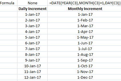
One of the more common date calculations in Excel is to increment your dates. If you want to increment a date by months, years, or days, then you can use the DATE function to do so. This function has three arguments: year, month, and date. If I have a date in cell C3 and I want to make cell C4 one month later, I would use the following formula:

=DATE(YEAR(C3),MONTH(C3)+1,DAY(C3))

For each of the year, month, and day arguments I used their individual functions. The YEAR function will take the year of the date specified, as the MONTH function will take the month, and the DAY function will take the specific day. For the DAY and YEAR functions I simply just referenced cell C3 since I want those values to remain the same. The MONTH function also took the same value from cell C3, however, I added +1 to it as well to increment the value by one month.

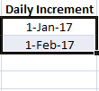
If I want to just increment by day, then I can just enter a starting date and drag that value down, and Excel’s autofill will automatically increment the values by one day. Here’s a comparison of the daily increment (where no formula is necessary) and the monthly increment, where I use the formula noted above:

Incrementing dates by month using a formula vs autofill.

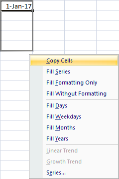
Now, there is another way, an even simpler way, just by using Excel’s autofill feature that I can increment by month. If I enter my starting date in cell B3 and pull it down using the fill handle, Excel will increment by day. However, if I select cell B3 and pull down the fill handle while also holding down the right-click button, it gives me the option to select how I want to increment – including fill days, weekdays, months, and years.

This way you can ensure Excel increments as you like. If you just use the fill handle without the right-click button you don’t get these options and Excel fills in the data how it thinks makes sense. Interesting to note that if you fill in cell B4 with the next month, and then select cells B3:B4 and then use the fill handle, then Excel has figured out you want to increment by months and doesn’t increment by days anymore. The more of a pattern you show Excel, the more likely it will know what you are trying to do.

incrementing dates

In the above picture if I now double click the fill handle my daily increment will become monthly since I have selected two points in my series. And since the two points have a monthly interval, Excel assumes I want the rest of the series to also have monthly intervals as well. The result becomes this:

You may wonder what the point would be of using the date function in the formula above if you can just use the fill handle since it is faster and easier. The main benefit of using a formula is if you don’t want to have to use the fill handle all the time. If you just need to set up your dates one time, then certainly the fill handle makes sense. But if you are working with a large data set that you will continually add to, you might find it a bit easier to have a formula there as opposed to using the fill handle each time and making sure it is incrementing correctly.

Calculating the Difference From/To Today

If you want to include today’s date in your calculations, you can use the TODAY() or NOW()functions. These functions have no arguments and you just enter them with both parentheses. This will generate today’s date. The difference between the two functions is the NOW() function also includes the time. But for the purpose of calculating the difference in days, either one will do the job.

NOW() and TODAY() Functions

Alternatively, you can use the shortcut CTRL+; which will plug in today’s date. If you want the date to update every time you open the spreadsheet then you are better off using the functions. If you want to do a one-time insertion of the current date never to change later, then the shortcut will do. It is no different than just entering the date yourself.

End of Month Calculations

Suppose I wanted to not calculate the number of days from today, but the end of the month. What I could use is the EOMONTH function. This has two arguments – start date, and months. If I wanted to use the end of the current month, I would enter the following formula:

=EOMONTH(TODAY(),0)

If I wanted the end of next month, then I would change the 0 to a 1:

=EOMONTH(TODAY(),1)

The months argument just tells Excel how many months ahead to go. Whether you change the months argument or alter the start date to get to a later month end value, it doesn’t matter, both methods can get you to the desired result.

EOMONTH Function

Calculating Workdays

Up until now, I’ve gone over how to calculate the difference in days. But suppose I wanted to calculate only working days. To do this you can use the NETWORKDAYS function which will take the starting date, ending date, and calculate how many workdays fall in between. To be more accurate you could also include a list of holidays into the function (which you will have to populate).

NETWORKDAYS Function

In the above example, I selected Jan 2 and 3rd as holidays so as a result, the NETWORKDAYS function with holidays has two days fewer than the function without holidays since those days both fall within the date range. Without a list of holidays, the NETWORKDAYS function effectively calculates weekdays since it would only ignore weekends. Also note that in the argument for holidays, do not include any text fields such as a header for holidays. If my range included the header then it would return a #VALUE error.

A similar function, WORKDAY takes the starting date, and you select how many workdays you want to advance by, and it will return a date result for the next working day after the days you specified. Again, you can list the holidays to ensure a more accurate calculation.

WORKDAY Function

If you don’t use holidays then both functions (NETWORKDAYS and WORKDAY) will not adjust for them. However, both functions will recognize and skip over weekends and so if you leave holidays blank they effectively just look at every weekday.

Calculating Weeks, Months, Years

If I wanted to do date calculations in Excel to show the difference between two dates in weeks, what I could do is use the WEEKNUM function and then use my date as the argument for that function. Once I calculate this for both dates then I just calculate the difference. This strictly looks at the week of the year, so it won’t take into account whether one date is a Friday and the other a Monday.

WEEKNUM Function

And if you wanted to you would be better off dividing the difference in dates by 7 to get fractional weeks.

For months you can do the same thing, except using the MONTH function which will yield a result from 1 to 12. The YEAR function will do the same as the month function, give you the year of the specified date, which you then can use in your calculations to calculate the change in years. You can also use the YEARFRAC function if you wanted to calculate the difference in fractions of a year, to give you a more specific result when calculating the difference in years.

YEARFRAC Function

Formatting Dates

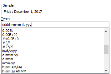
In addition to just doing date calculations in Excel, it’s important that your dates are also formatted properly. You can format dates so they display exactly how you like right through the format cells option. The easiest way to do that is to go to the cell formatting (right-click format cells, or click ctrl+1), and select the CUSTOM category.
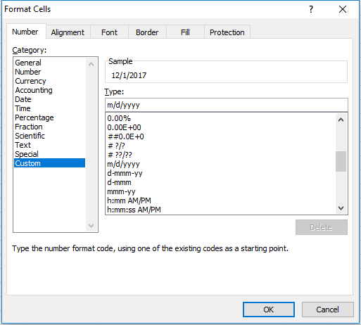
Custom Date Formatting

If you want month/day/year (which it may already be set to) the formatting is just m/d/yyyy. But what if I didn’t want to show all four numbers for the year, just the last two? Then I would set it to m/d/yy. You can flip the d and the m around so it is d/m instead of m/d and then you have day/month/year. If you use two d’s rather than one you will get a 0 if you are in single digits for the day. For instance, instead of 1/1, you could get 01/01. You will notice the changes in the sample box above as you change your custom category.

Here is  a quick summary of the use of letters and what results they will yield:

  • m or d: will use 1, 2, 3, etc.
  • dd or mm: will use 01, 02, 03, etc.
  • ddd or mmm: will spell out the abbreviation (e.g. ‘Mon’ for Monday, or ‘Nov’ for November)
  • dddd or mmmm: will spell out the entire day or month (e.g. Monday, November)
  • y or yy: will use the last two digits of the year.
  • yyy or anything more: will use the full four digits of the year.

If I wanted to use a formal date that showed the day and month spelled out, followed by the numerical day, a comma, and the year, I would use the following format:

dddd mmmm d, yyy
Date Format


If you liked this post on How to Do Date Calculations in Excel (and Format Them), please give this site a like on Facebook and also be sure to check out some of the many templates that we have available for download. You can also follow us on Twitter and YouTube.

Forecast

Shading Areas on a Chart to Highlight Gaps and Variances

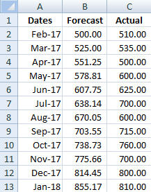
When comparing forecasted amounts vs actuals one way to help emphasize and highlight variances is by shading those areas. I’ll show you how to easily do that in this post.

Below is my starting data set

Forecast
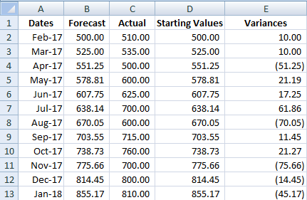
I will need to create two extra columns to this data set. The first one I will just call Starting Values and they will match my forecasted amounts. The next column, called Variances will be equal to the actuals less forecasted values.
Variances
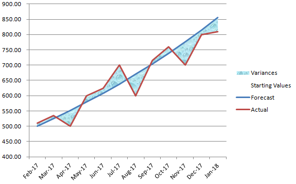
Next I will plot a line graph with these values. 
line graph
I will need to change the chart type for the starting values and variances data sets. They need to be set to the stacked area charts.
Area charts
For the starting variances series, click on Format Data Series and under the Fill section select No Fill. What remains are the shaded areas in addition the line graphs. You can change the shading to a different fill colour or texture.
shaded chart
horizontal line data

Plotting Vertical and Horizontal Lines in Charts

When charting something on Excel you sometimes may want to add vertical lines to identify key dates, or horizontal lines for target or benchmark amounts. In this post I’ll show you how to do both.
Horizontal lines can be used to identify target or benchmark amounts while vertical lines are useful to mark dates. In my example I’ve downloaded googles historical closing stock prices for the year and I’m going to mark the year long average and identify their earnings dates

Horizontal Lines

I’ll first start with horizontal lines. If you have amounts on the y-axis then a horizontal line can act as an indicator to show if the amounts have crossed a targeted amount. In order to add a horizontal line all you’ll need to do is create another column in your table.
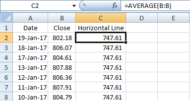
The key thing for this column is all the values have to be identical for each entry. I can set it to a single number and copy it down, or I can do a calculation as well. What I will use is the closing price average in this column using the AVERAGE formula. If I copy this down I am left with a value that stays constant for the entire data set.
horizontal line data
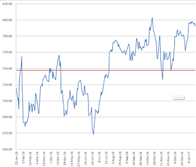
If I chart this graph using a line chart my horizontal line is now visible
chart horizontal line

Vertical Lines 

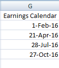
Vertical lines are a bit more tricky but not difficult. In my example I am going to put a vertical line at every earnings date since I know those days will have a lot of fluctuations and will also create quarterly intervals. I have created a column for all the earnings dates in the year, aka my earnings calendar.
earnings calendar
 Again I will need to create another column in my table. 
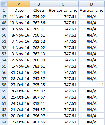
In this column I will look to see if the date for this row matches one of the dates in my earnings calendar. If there is a match, I will set the value to 1. Whether you use the MATCH formula or the VLOOKUP formula doesn’t matter. But I will use the MATCH formula in this example. The key is including the IF and ISERROR formulas  because if I do not find a value it will return an error, and specifically I will use the NA() formula to return the NA error so that that amount does not appear on the chart as a zero. And if it is a match, I can make it set to 1.
First I will start with the IF function, add ISERROR, and add the MATCH function to now see if the date on this row matches anything in my earnings calendar), and if it is not a match, make it equal to an NA error, otherwise make it equal to 1 indicate a match.
My formula looks like this:
=IF(ISERROR(MATCH(A2,G:G,0)),NA(),1)

Where column G is where my earnings calendar is located.
Now I will copy my formula all the way down. It may not look terribly nice in your table with all those errors but it will get the job done.
Match function
I’m ready to chart my graph now. Select line chart again. However unlike for the horizontal line, it needs some work.
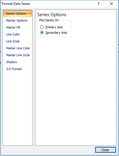
The earnings dates need to be plotted against the secondary axis. To do this, I right click on the series and click Format Data Series and select Secondary Axis.

Format data series

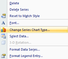
Next, I need to change the series chart type so that it is a column chart. I will right click on the series again and select Change Series Chart Type and then select a column chart.
column chart
I will go back to format the data series once more to add a border which will allow me to make the line look thicker.  By going to Border Colors this time I can specify the colour, and then under Border Styles I can modify the Weight.
I will now format the secondary data axis. I will set the maximum height equal to 1, the value that I set for the earnings column when there was a match. It doesn’t matter what you set that value to, whether it is 1, 100, 1000, you will just need to change the axis accordingly to make sure that value is at least as large as your scale to have the line go all the way across. If you have values that you are currently using on your secondary axis you will want to take that into account and consider what is a good maximum value for that secondary chart, and use that value, rather than 1.
Next, I will hide the secondary axis (if you need it for other values obviously this is optional). To do this right click on the axis, click Format Axis, and set Axis Labelsto None.
Axis Labels
Now my chart is good to go with both vertical and horizontal lines.
Chart Vertical Line
awater

How to Make a Waterfall Chart in Excel


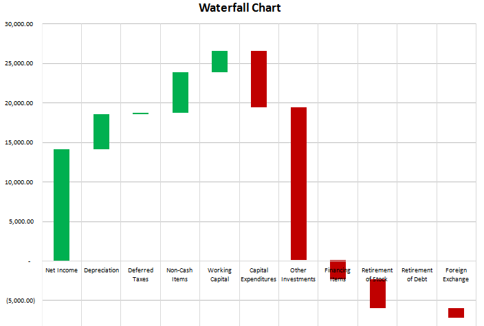
waterfall chart
This is a chart that is useful in reviewing variances and monitoring change from one period to another. Favourable (positive) variances are green, and unfavourable (negative) variances are red. In this example I used a statement of cash flow. Increases or inflows in cash are favourable, while decreases or outflows of cash are unfavourable.


On the data tab all that is required is the change column (B), and the remaining formulas can stay intact.

If you were to track the changes in an income statement, you want to be careful to make sure favourable changes are positive and unfavourable ones negative. For example, if sales are up 100,000, that should be favourable since it has a positive impact on net income. However if expenses are up 100,000 that is unfavourable since it has a negative impact on net income, so although it is technically an increase, the change should be negative. This is where the cumulative change column is helpful because it shows you the running balance, and the ending figure in that column is what you are reconciling to. If that number is not correct then you know somewhere a sign is wrong or an amount is missing.


The remaining columns (D:H) simply have to do with the appearance of the chart. Columns D:E are positive changes, G:H are negative, and F represents the amount that is not visible or blank. The purpose for the blank values is what allows the waterfall chart to create the effect of starting from the last position and just showing the change in the cumulative value.


Inventory count sheet showing data by product number.

How to Sort Data in Excel Without Messing Up Formulas

If you have a formula that involves multiple sheets and you later sort that data you may notice your cell references are now out of order and need to be corrected. It can be frustrating and dangerous because you may not realize your formulas are now calculating different cells.

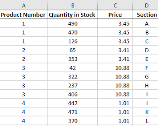
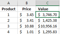
For example, I have created a sheet called InventoryCount and another called Total. The InventoryCount sheet acts as a tally of all the locations a certain product number is found:

Inventory count sheet showing data by product number.

On the totals sheet, I have a summary of these product numbers using a SUMIF formula that multiplies by the price.

A summary of the inventory values.

The formula in the highlighted cell above is as follows:

=SUMIF(InventoryCount!A:A,Total!A2,InventoryCount!B:B)*B2

The formula in the price column for product 1 is:

=VLOOKUP(A2,InventoryCount!A:C,3,FALSE)

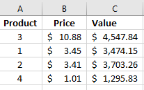
Both formulas are referencing the InventoryCount sheet. The formulas in the value column are correct. But let’s say that I want to sort that column by values. If I sort in descending order, this is what I get:

Inventory data after applying a sort.

The values are not only not correctly sorted  (product 1 is lower than product 2’s value) but the values have changed. If you look at the values before the sort product 3 dropped from 10,956.16 to 4,547.84. There is nothing glaringly obvious that the calculation is now completely incorrect so you can imagine the danger when dealing with lots of data that such a sort could make your data get altered. The formula for the value in product 1 now looks like this:

=SUMIF(InventoryCount!A:A,Total!A2,InventoryCount!B:B)*B3

It is still referencing A2. So technically the formula is still correct, the problem instead is product 1 is no longer on row 2, it is on row 3. The assumption that the value in row 3 relates to the product on row 3 will now be incorrect.

So why did this happen? Notice that the price has not changed for any of these products, Product 1 was $3.45 before the sort, as well as after. This column still is correct in relation to its corresponding products.

If you go back and look at the two formulas (price and value) you will notice on key difference: the cell referenced on the current sheet (Total) for the price does not mention the sheet name, however on the value formula it does.

This is the original formula to calculate the value:

=SUMIF(InventoryCount!A:A,Total!A2,InventoryCount!B:B)*B2

The Total! reference is causing the sorting issue and needs to be removed. The updated formula becomes:

=SUMIF(InventoryCount!A:A,A2,InventoryCount!B:B)*B2

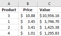
Now if I apply the same logic to the other formulas in the value calculation and sort the data in descending order, below is the result I get:

Inventory data after applying a sort.

The values are back to what they were at the start and product 3 is the highest as it was initially. Except now they are correctly sorted in descending order with the product number correctly being referenced in column A.

So the lesson here is that if you are using formulas with multiple sheets get rid of the sheet reference when referencing a cell on the same sheet as the formula is on (Excel inserts this reference automatically as you switch from one sheet to the next). Otherwise, if you or anyone else sorts the data the calculations will not be on the correct rows.


If you liked this post on How to Sort Data in Excel Without Messing Up Formulas, please give this site a like on Facebook and also be sure to check out some of the many templates that we have available for download. You can also follow us on Twitter and YouTube.
Ranks in Excel: Breaking Ties

The RANK() function in Excel is limited to a single range and if you do not have a set of unique numbers to use the rank function on it will return repeating values.
There is a workaround however. If you can afford an extra column for a ‘rank total’ then it will be easy to accommodate. Or you can use an array formula.
The easiest example in creating a rank total column is to look at standings in sports:
Team
W
Points
GF
GA
Goal Differential
Team A
5
15
20
5
15
Team B
4
12
19
18
1
Team C
6
12
12
7
5
Team D
4
11
17
15
2
In this scenario I’m going to say the rank order will first be by points, the first tiebreaker will be wins, followed by goal differential. My rank total formula will be as follows: Points + wins/100 + goal differential/10,000. I’ve broken out how the values look and after totaling them:
Team
W
Points
GF
GA
Goal Differential
Win Value
Differential Value
Rank Total
Team A
5
15
20
5
15
0.05
0.0015
15.0515
Team B
4
12
19
18
1
0.04
0.0001
12.0401
Team C
4
12
12
7
5
0.04
0.0005
12.0405
Team D
4
11
17
15
2
0.04
0.0002
11.0402
For Team A, their rank total is made up of 15 (points), .05 (wins) and .0015 for goal differential. If the factor for goal differential was only 1,000, then goal differential adds 0.015 and now it affects the decimal position for wins and has the same effect as a sixth win, which is wrong. So you want to choose your factors carefully so as not to effect the higher ranking tiebreaker. If goal differential was only ever single digits then you could have used a denominator of 1,000 instead of 10,000.
The result of this rank total tells me Team C should be ranked higher than Team B because both teams have the same points, same wins, but Team C has the higher goal differential.
Now what you can do to pull the ranks is use the following formula:
RANK(ranktotalvalue, ranktotalcolumn)
Or if you want to put the name of the teams in order of their rank rather than just saying Team A is in position 1, then you can use the index and match functions as follows. Assume the Team column is column A and the rank total is column I:
=INDEX(A:A, MATCH(LARGE(I:I,ROW(A1)),I:I,0))
Let’s break down this formula:
=INDEX(A:A
This tells the formula I want to extract the value from column A.
LARGE(I:I,ROW(A1))
This extracts the largest value in column I. The reason I use ROW(A1) instead of the number one is because now if I drag this formula down the relative reference will become ROW(A2), ROW(A3), and ROW(A4) which then looks for the second, third, and fourth largest values respectively.
MATCH(LARGE(I:I,ROW(A1)),I:I,0)
This formula looks for where the value matches the result of the large formula calculation. Where that match is made, the related value from column A is returned. And the following list is generated:
Team A
Team C
Team B
Team D
This correctly puts Team C ahead of Team B in the rankings.
WHAT IF I DON’T HAVE ANY TIEBREAKERS?

If you do not have any tiebreakers then what you can do is pull them in the order that they appear. If you want them to be in ascending or descending order, then you will first need to sort the data in such a way.
In this case, you can calculate your rank total using a value for the row the values are on. The formula for the ‘row value’ would be calculated as follows: 1/(ROW()*100).  The fraction is used to make sure the rows higher up will appear first. I multiple the denominator by 100 to push it further down the decimal location. Below is how my rank totals now look:
Team
W
Points
GF
GA
Goal Differential
Row Value
Rank Total
Team A
5
10
20
5
15
0.005
10.005
Team B
4
12
19
18
1
0.003333333
12.00333333
Team C
4
12
12
7
5
0.0025
12.0025
Team D
4
11
17
15
2
0.002
11.002
I changed Team A’s point total to 10 for the sake of this example. Now the top two ranked teams (B and C) both have 12 points. Because B is in a higher row and thus shows up before C, it has a higher row value which in turn gives it a higher total rank value. So the correct order now is Team B, Team C, Team D, and Team A.
THE FORMULA METHOD

Now if you don’t have the luxury to put an extra column in your worksheet, you can certainly do this in a formula, although it won’t be pretty. Essentially you’ll recalculate the rank total and search through the values using an array formula.
To recalculate the rank for the non-tiebreaker method:
{=INDEX($A$2:$A$5,MATCH(LARGE(($C$2:$C$5)+(1/(ROW($G$2:$G$5)*100)),ROW(A1)),$C$2:$C$5+(1/(ROW($G$2:$G$5)*100)),0),1)}
The INDEX formula again looks at the Team column while looking for the largest value when adding the points value to the row value. The calculation for the row value is the same as above just now dumped into a formula. An array formula has to be used to ensure each team’s results are looked at individually.
For the multiple tiebreaker scenario from above, the formula will be longer to accommodate for all the extra tiebreakers it has to look at:
{=INDEX($A$2:$A$5,MATCH(LARGE(($C$2:$C$5)+($B$2:$B$5/100)+($F$2:$F$5/10000),ROW(A1)),(($C$2:$C$5)+($B$2:$B$5/100)+($F$2:$F$5/10000)),0),1)}
Again, same logic and formulas are involved except without a rank total column it has to be done in an array. The results yield the same order as through adding an extra column.

Removing Blank Spaces

When copying data into Excel from other sources – be it web pages, documents, or other Excel documents sometimes you end up with unwanted formatting, such as numbers with invisible spaces that prevents it as being read as a number or converted into one. Or just ending up with data you don’t want.
The TRIM function in Excel is useful for removing trailing spaces after text that serve no purpose.
The more annoying issue that I’ve come across is a blank space that looks like one but isn’t. It is usually character # 160 which looks just like a blank space, only thinner than normal. If you enter char(160) in a cell you’ll see what this looks like. It can be a frustrating process because this character you can’t get rid of by just searching for blank characters and doing a find and replace or the trim function. It’s possible to see this with other characters as 160 isn’t the only one that looks like a blank space, but it is the only one I’ve come across so far.
The solution is to replace character 160 with character 32 (this is a normal space that will get eliminated with the TRIM function). To do this, use the following formula, assuming cell a1 is the cell that needs the cleanup:
=TRIM(SUBSTITUTE (A1,CHAR(160),CHAR(32)))
You can add a *1 to the end of the formula to convert it to a number if necessary.
See below for an example. The only difference between the cells in A2 and A3 is A2 has a normal blank space after it whereas cell A3 has character 160 after it. Both cells equal the same length (12 characters) as show in column B. column C is what the cells look after using the TRIM function – they will look the same but column D recalculates the length and the top cell has now gone down by one character (the trailing space). Column E is after the above formula is used. You can see now the updated length in column F is 11 for both, meaning the trailing character has been deleted in both cells.

As a side note, if you’re need to reference a specific character in excel you’ll notice all it takes is using the CHAR formula. If you’re not sure which number of the character you need, you can have the CHAR function reference the numbers 1 to 255 and you’ll see all the different characters available.

Convert LAST NAME, FIRST NAME into different formats

In many databases names may show up as last name, first name which doesn’t make it ideal for sorting and filtering data easily. However this can be quickly rearranged in Excel. I’ll show you two ways to do this: 1) using text to columns (the easier method) and 2) using formulas

1) Using Text-to-Columns

Select the cells that have the last name, first name format and under the Data tab click on Text to Columns.

On the popup that comes up select Delimited and click Next

On the next screen, make sure Comma is the only delimiter selected and then press Finish

Doing this will put the last names in the current range and the first names in the adjacent column B. You will want to make sure the adjacent column is blank to make sure you don’t accidentally overwrite data that may be in those cells already.

An optional step, if you wanted to combine both last name and first name into one cell is to use the following formula in cell C18:

=B18&” “&A18

B18 is the first name and A18 is the last name fields. The ampersand connects the words with a blank space inbetween. Cell C18 would show John Smith

For Excel purposes, it’s probably ideal to have the last name and first name in separate cells rather than in one.

2) Using Formulas

Extracting the Last Name

First, the formula to extract the last name (assuming the cell is A2):

=LEFT(A2,FIND(“,”,A2,1)-1)

If I have Smith, John in cell A2, then the result is as follows:

The LEFT function extracts x number of letters from the left of the cell. The key is the second argument. It consists of:

FIND(“,”,A2,1)-1

The FIND function looks for a comma within cell A2, and begins at the 1st character. If the cell is Smith, John then the comma would be found in the 6th character of that cell. The -1 that is after the FIND function is to reduce this to the 5th character. This is done because I don’t want to include the comma in the name.

So how the LEFT function works is from cell A2 it pulls the first 5 characters from the left, which will result in Smith

Had I not included the -1 after the FIND function, it would have been Smith,


Extracting the First Name

Now I’ll show you how to extract the first name using a similar function, the RIGHT function:

=RIGHT(A2,LEN(A2)-FIND(“,”,A2,1)-1)

The logic behind the RIGHT function is the same as the LEFT function, except this time the formula pulls the characters from the right instead of the left. However you’ll notice the second argument is a little more complex this time. The argument is as follows:

LEN(A2)-FIND(“,”,A2,1)-1

The key difference is I am now using the LEN function which tells me the number of characters that are in the cell. LEN(A2) would return 11 characters for Smith, John

Why can’t I just use the RIGHT function the way I used the LEFT one? The reason being is the FIND function searches from left to right and not from right to left, so it will tell me the position of the comma from the left, not from the right. So if it returns the number 6, I know the comma is the 6th character from the left, but doesn’t tell me how many from the right.

In order to do this I have to use the LEN function. If the total cell is 11 characters long, and the comma is at the 6th character, that will mean there are 5 characters after the comma. Coincidentally in this case the comma is 6 spots from both the left and right, making it right in the middle of the cell.

Here again I use the -1 after the FIND function because if I pull the 5 characters from the right, it will include a blank space (obviously if the data is formatted as last name,first name instead of last name, first name you can omit the -1).

Combining the Two

Now these two functions have allowed me to pull the different parts of the name out of a comma separated last name, first name format. If you want all of this into one formula (and assuming you want first name last name to be in a single cell) then all you would need to do is enter the formula as follows:

=RIGHT(A2,LEN(A2)-FIND(“,”,A2,1)-1)&” “&LEFT(A2,FIND(“,”,A2,1)-1)

I’m reusing the formulas used earlier and connecting them with ampersands while also adding a space inbetween.

Referencing Cells in Other Worksheets and Workbooks using the INDIRECT function

When working with multiple worksheets or tabs, it becomes useful to reference them in formulas or to consolidate data. First, I’ll look at working with different tabs.
Referencing Other Tabs

The easiest way to refer to a cell in another tab is to start a formula with the = sign, and then click over to the other tab and click on the cell you want to reference.  In the following example I am typing a formula in tab A but will reference cell B6 on tab B.
Note the reference in the formula bar:
=B!B6
The tab is denoted by the ! after the tab name. If I wanted to reference tab A it would look as follows:
=A!B6
But what if my tab wasn’t all one word, and the tab was named A and B? In this case, I would need to use apostrophes:
=’A and B’!B6
So to summarize, the naming convention for referencing another sheet is:
SHEET1!A1 or ’SHEET 1’!A1


Linking to other Spreadsheets

Now let’s assume the cell you want to reference isn’t in this same workbook, then the reference looks a bit different. If the workbook is open:
=[Workbookname] SHEET1!A1

The key difference is you are adding the workbookname. This method will work if the workbook is open, but not recommended if you are referencing a workbook that is closed because Excel might not know which workbook you want to reference and cause errors. To properly reference a closed workbook, use the following:
=’C:Desktop[Workbookname.xlsx]SHEET1!A1
The above formula will work if the workbook is saved on my desktop.
In this example I only used a single cell, but you can just as easily reference a range. Change A1 to A1:A10 and you are referencing a range instead of a cell. This comes in useful if you want to use the reference in a lookup.
Using the INDIRECTFunction

Referencing other worksheets and tabs is not difficult once you get used to the syntax, but if you had dozens of tabs or workbooks you wanted to reference, it might get tiresome to keep doing this. That’s where the INDIRECT function comes in handy. You can use formulas to populate these cell references so that you don’t have to re-type them or even use find and replace.
Imagine you have sales data on multiple tabs. Each tab represents a year. So if I want to summarize data from five different years (tabs), that’s five different references I have to use. Or I can use the INDIRECT function. The way the formula works is you can enter the entire location of the cell that you want to reference. The benefit is being able to use relative and absolute references in place of having to type out the full address over and over again.
Here is a comparison of how the references would look using each method:
In the indirect function, I am able to use a relative reference for the year. If I enter the formula in cell B4, all I have to do is copy the formula down and it will reference all the other years(tabs) without having to re-type the full location. The benefit here is apparent when you are dealing with many different tabs. In column C I am unable to do this and have to re-key each cell individually.
The tricky part of using the indirect function is making sure you are correctly combining the ampersands, variables, and constants. The ampersand you use to join a constant and a variable within the INDIRECT formula. In this example, the variable is the year (tab name). The constant is the syntax (!) and the cell reference (A1), since their values will never change.  Never put the variable in quotations, only constants. 
Here is a breakdown of the logic of the formula in cell B4:
Because I am referencing another tab (not another workbook), I need to start with the worksheet name. Since I have a variable for the worksheet name, I start with the reference to cell A4, which contains the name of my worksheet: 
=INDIRECT(A4
The remainder of the formula is going to be !A1, or, the constants. To add the constants, I need to add the ampersand, open quotations, enter the constants, and close the quotations and the formula:
=INDIRECT(A4&”!A1”)
You can alternate between constant and variable as much as you like but they have to be linked by an ampersand. You also don’t need to begin the INDIRECT function with a variable, it can be a constant.
Using INDIRECT with Workbooks
You can use the INDIRECT function to reference other workbooks, but unfortunately a limitation of the formula is that it is unable to get data from a closed workbook. So unless you plan to have the workbooks open, the formula will not be of much help here. The formula is most helpful when dealing with multiple tabs in a single workbook.
Avoiding Errors

Some key things to remember when referencing other sheets or workbooks:
  • Syntax is important, like in all formulas, but in these cases it’s very easy to make an error. Remember the !  comes right before the cell reference, and in the case of other workbooks, ‘! precedes it.
  • The INDIRECT function will help expedite referencing other tabs, but cannot help you with referencing closed workbooks.
  • If your tabs do not follow a consistent, predictable pattern then a formula won’t be able to help you much
  • You won’t be able to get data from closed workbooks that are password protected
  • Don’t forget the extension. In my example it was .xlsx but it may be different depending on your version and type of file.

How to Create a Named Range in Excel

Naming ranges offers an easy way to refer to a single cell or range without having to remember the address, and instead referring to it by name instead. This comes particularly useful if you will continually be referring to that cell. 
The key advantages of using named ranges:
– Less time consuming to find a named cell
– Easier to put into formulas
– Easier to reference in VBA
– Easily inserting hyperlinks in documents

Creating Named Ranges


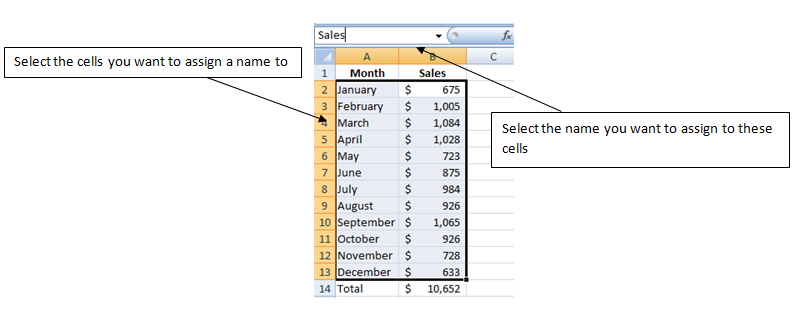
Below I have sales data listed by month. If I wanted to reference total sales I would need to refer to cell B14.
Let’s say this sheet is just one of many, and these are sales for product A.  The more products I have, the more useful it becomes to have named ranges, otherwise I would have to either a) remember the location when typing a formula, or b) navigating to the cell I want to reference. By using a name, it is easier to recall and doesn’t take much effort to include in a complex formula that may include many references.What I could do is name cell B14 as ProductASales (and subsequent ones could follow the same patter – ProductBSales, ProductCSales, etc..)
All I do is select cell B14 and type ProductASales in the cell reference that previously had B14. B14 still exists, but now I can reference the cell by just typing in ProductASales as well.
A range can have more than one name. If you want to delete or edit a name select the Name Managerunder the Formulas tab
I find that I have created two names for the same range. To delete one I just select the name I don’t want and click Delete. Now if I just wanted to change the range I can click Edit

There I can change the range to whatever I want.
Named ranges can also be used for multiple cells in the same way.

Note that a named range will move as a relative reference. If you insert or delete rows the name will move along with your cells. It can also expand, just like any other range in Excel. If for instance you insert a row between May and June, that will add that row to the range. Instead of including the cells from A2:B13, it will now include the cells from A2:B14 – since December will be pushed down to row 14.

Now that the ranges are setup, they can be referred to in a formula.

In cell H8 you can see that I entered a formula consisting only of the named range ProductASales. Instead of referencing cell B14 I can use this name.
This won’t work the same way for the Sales range since it relates to more than one cell. However, I can use it as part of a formula, vlookup for example:
Here I am using Sales as a table. Instead of typing out the full range A2:B13 I only have to type in Sales.

Apply Named Ranges to Existing Formulas


But let’s say you didn’t realize you could use named ranges and have been manually entering the ranges. You can update your formulas so they reflect the named ranges by doing the following:
Under the Formulastab, select Define Name, and Apply Names.
 At the following screen I select both names and press OK.
Now all my formulas with B14 or A2:B13 will be replaced with ProductASales, and Sales, respectively. This won’t affect your formulas in any way but now if you look at a formula you can easily see if it is referencing a named range.

Using Named Ranges in VBA


Another benefit of using named ranges is that it makes it easier to keep formulas consistent. In VBA, to reference these ranges, unnamed, would be as follows:
Worksheets(“Sheet1”).Range(“B14”)
Worksheets(“Sheet1”).Range(“A2:B13”)
The problem with this is that if you move the cells around, cut, copy, the references in VBA are absolute and will never update the way relative references in Excel will.  However, if you use named ranges, this problem is avoided. The reference would be as follows:
Range(“ProductASales”)
Range(“Sales”)
If you are coding in another worksheet, you will have to qualify which spreadsheet the named range is in:
Worksheets(“Sheet1”).Range(“ProductASales”)
Worksheets(“Sheet1”).Range(“Sales”)
Now if these ranges are moved within Excel, you don’t have to worry about updating them within VBA.

Named Ranges as Hyperlinks


By using a named range you can also easily add hyperlinks into your spreadsheet. For example, let’s say on Sheet 2 I want to link to the sales data:
On the Insert tab, select Hyperlink.
Select Place in this Document and you will see a list of the defined names. If I press Sales and click OK this will create a hyperlink in the active cell:
Now if I click on the Sales link in cell D6 it will bring me to the named range that belongs to Sales.