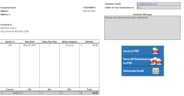
This is an updated version of a prior post that generated a statement without VBA, but the limitation there was you had to save the pdf yourself. This updated version allows you to do the following:
– Save the current statement to PDF
– Cycle through all your customers and save all their statements to PDF
– Generate an email (but not send) to the customer with the attached statement.
It is important to note the customer name on the invoice data needs to match the name on the customer data tab otherwise the invoices will not pull on the statement correctly.
The template works in exactly the same way as the prior version – invoice data and customer data needs to be downloaded from your accounting software. You can customize your statement and include any images you like so that it will look consistent for every statement that you send out.
This template is setup to accommodate up to 150 invoices.
In many cases it is inefficient to run one long sub procedure in VBA. Rather, it is easier to break them up into smaller processes. I’m going to show an example of how to do this using a simple square root function, and having a variable passed from another sub procedure.
My initial subprocedure will just assign a test value, use the square root function to determine the square root, and then return a message box to summarize the results.
————————————————————————————
Sub test()
Dim testvalue as Integer, root as Integer
testvalue = 25
root = sqrt(testvalue)
Msgbox “the square root of ” & testvalue & ” is ” & root
End sub
————————————————————————————
The root variable comes from the sqrt function which is below:
————————————————————————————
Function sqrt(cl as Integer) as Integer
sqrt = cl ^ 0.5
End Function
————————————————————————————
The sqrt function takes the cl to the power of 1/2; its square root. The sqrt function requires a variable for it to work, which is indicated by the parentheses, indicating that it requires the cl variable to be an integer. That is the key requirement, that the variable passed to the sqrt function is the same data type.
The sub procedure at the top assigns 25 to the testvalue variable. The next line calls the sqrt function and uses the testvalue variable as the argument for the function. Effectively it is going to calculate the square root of 25. This result will be assigned to the root variable. The last line before the end of the sub procedure simply pops up a message box to say what the square root of the testvalue is.
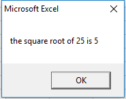
If I run the first sub procedure this is what the message box results in:
As you see the square root of 25 is indeed 5, so the calculation worked correctly.
However, let’s pretend my function has an additional line where it sets the cl variable to 9:
————————————————————————————
Function sqrt(cl as Integer) as Integer
sqrt = cl ^ 0.5
cl = 9
End Function
————————————————————————————
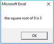
Now when I run the sub procedure the message box I get is this:
Obviously this is not correct. And you’ll notice that now my variable in my sub procedure has been changed to 9. The reason for this is because the variable has been passed to the function by Reference, or ByRef. As a result, when the sub procedure sends the testvalue variable to the sqrt function, the testvalue variable effectively assumes the cl variable, and when the cl variable is changed to 9, when the variable is now sent back to the sub procedure it is with the value of 9. Sending a variable by reference allows for the variable to be changed by the function.
The other way to pass a variable is to pass it by Value, or ByVal. Becuase ByRef is the default in VBA, it does not have to be stated. But to pass it ByVal that needs to be specified. Below is the adjusted function now taking only the value rather than the reference:
————————————————————————————
Function sqrt(ByVal cl as Integer) as Integer
sqrt = cl ^ 0.5
cl = 9
End Function
————————————————————————————
Now when I run the sub procedure I get the following message box:
The calculation reverts back to the correct message I had initially before I added that line of code to change the cl variable. But even with the change in code, by setting the variable to ByVal, it ensures my original variable cannot be changed in the sqrt function.
Doing loops in VBA is very useful because it allows you to go through a range of cells, evaluate each, and then take an action if a specified criteria is met. I am going to go through a couple of examples to show you how you could do this to highlight cells and also delete rows.
For a brief intro to macros check out my earlier post about how to access VBA and record macros.
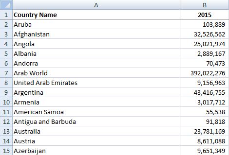
I have a data set below that shows population by country in the year 2015:
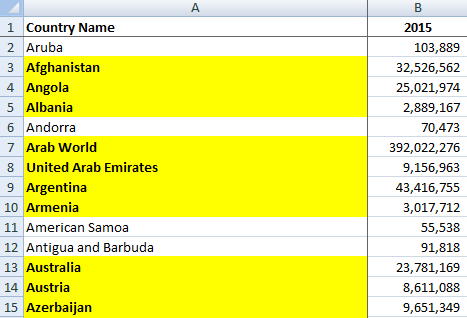
First, what I will do is do a loop to evaluate each country’s population for 2015, and for any that had more than 1,000,000 people, highlight the country name in column A.
There are a number of ways to do loops in VBA but I prefer using the For…Each loop.
The key thing is first to define the range of cells I want the loop to be applied to. I can use Excel’s COUNTA function to count the range. To do so, I first setup a variable called totalcount:
WorksheetFunction allows me to use Excel functions that are accessible in a normal spreadsheet and are accessible without VBA, in this instance, COUNTA. The totalcount variable now tells me how big my range needs to be; to what row I need my loop to go to.
I created a couple of additional variables as well: cl – this is the specific cell that will be evaluated when the loop is in progress; ws – this is just the worksheet which allows me to shortcut having to spell out the name of the worksheet each time (in this case it is just the default Sheet1). Below are my variable declarations:
The first line in my loop specifies the range that I am going to cycle through:
For Each cl In ws.Range(“A2:A” & totalcount)
The above can be interpreted as saying that I am going to cycle through each cell from the range A2 until A and whatever the totalcount is equal to. I have to close the loop as well, so the last line of the loop is as follows:
Next cl
The point of the above line is that once I finish evaluating the cell and making whatever changes I need I now move onto the next cell to evaluate. This variable does not have to be called cl, it just makes it easier to think of instead of next a or b let’s say.
So that is the loop. But without anything inbetween the start and end of the loop all the sub procedure is going to do is go through every cell in that range and do nothing. So as mentioned I want to determine if the population is more than 1,000,000:
If cl.Offset(0, 1) > 1000000 Then
I use the offset function to evaluate the column adjacent to colum A. I could have selected my range as being B rather than A and I wouldn’t need to do an offset. However, using offset(0,1) tells the procedure to look at the column to the right. Just like the regular excel function, the first argument in the offset function is the number of row offsets, and the second is the column offset. So the above line evaluates if the related value in column B is more than 1,000,000. The next line I enter is what will happen if it is true:
cl.Interior.Color = vbYellow
This will highlight the cell in yellow. There are a lot of things you can do and in VBA once you type the period after your range, in this case once I enter cl. it will show me a list of properties and methods that I can use. It makes it easy if you don’t remember the exact property or method name:
If I wanted to make the cell bold I would do the following:
cl.Font.Bold = true
I did not use the offset function here as I want the country field in column A to be highlighted and bolded. My entire sub procedure from start to finish looks as follows:
The above code will work in the exact same way as the previous, the only difference is the counter. You’ll see in the below examples why a counter is useful.
Suppose I wanted to delete the rows where the population was less than 1,000,000 people in 2015. I could modify my original code to work as follows:
The key difference is instead of bolding and highlighting I have the following line:
cl.EntireRow.Delete
This line will delete the row that the cell is on. If I run this subprocedure, I get the following result:
You’ll notice there is a problem. I have a country that has less than 1,000,000 people in this list – Antigua and Barbuda. It worked in a few instances – it got rid of Aruba, Andorra, and American Samoa. The problem is because American Samoa was right before Antigua and Barbuda. When I delete a row the loop does not factor in that the row that Antigua and Barbuda was on has now moved up a slot so when the loop goes to the next row it has skipped over the one that Antigua and Barbuda is on. So the loop fails in this instance when you run into consecutive rows meeting the condition you have specified.
However all you need to do to correct this is to start your loop backwards: start from the last row and work your way up. To do this I use the counter, The opening line of my loop is as follows:
For counter = totalcount To 2 Step -1
If you recall totalcount is my last row, and it will go until it reaches row 2. Step -1 indicates that it should go up one row at a time (if I wanted it go up two rows at a time it would be Step -2 instead). That way if I delete a row it doesn’t affect my loop since the data above the row I’ve deleted remains the same. My new sub procedure looks like this:
PLEASE NOTE THERE IS A NEWER VERSION OF THIS TEMPLATE AVAILABLE HERE
A bank reconciliation can be a time-consuming process but this template can help speed it up. By assigning categories and setup quick ways to match items, you can quickly accelerate the reconciliation process. With an easy interface to match transactions, this template should help speed up what can otherwise be a tedious process.
Download Options
This version has been discontinued. Instead, please refer either to the 2020 or 2023 versions.
Note on #NAME? Errors
If you see this error message in the spreadsheet it means you have not enabled macros when opening the file or the calculations have not been able to update. If you think macros have been enabled and updated calculations but don’t see the results updated, then just try re-opening the file and that should fix the issue.
How to Use This Template
This template allows you to easily reconcile your bank to your book by 1) categorizing transactions, and 2) reconciling any matches based on those categories.
Setting up Categories to Match Transactions
In order to categorize transactions, you will need to use the Setup tab to first create the rules that will find and identify categories. The setup tab has five columns: Category, Identifier, Key, Length of Key, and Gap.
The Category column is simply the name of the category (e.g. wire transfers, deposits, cheques).
The Identifier is what needs to be in your transaction description to be flagged as belonging to this category. For example, suppose the following description on your bank statement indicates cheque # 1234 was cashed:
C#1234
In the above example you would want to set C# as your identifier since that is how you can identify this is a cheque and should belong to the cheque category. The category can have multiple rules (for example, the way a cheque is indicated on your bank is likely not the same as on your general ledger)
The next column, the Key, is what should be used to try and match and reconcile these types of transactions. This is a drop-down selection as there are multiple options: use date, use letters after identifier, use numbers after identifier, and use alphanumeric string after identifier. You can also leave this blank if you don’t want the template to try and automatically reconcile these transactions or if there is no discernible key that can help identify the transaction.
To use the date will mean just the date is used, nothing else. In the case of a cheque this will not work since you might have multiple cheques deposited in a single day, so to just look at date will not correctly reconcile these types of transactions.
In the case of cheques you will want to select ‘Use numbers after identifier’ since that will pull only numbers and not any text. If you need text you can select the option for ‘Use letters after identifier’, or if you need both numbers and letters – ‘Use alphanumeric string after identifier’
The Length of Key column is how long you want the key to be. Suppose the following description:
C#12340000000
Although the cheque number is 1234 the description leaves trailing numbers afterward or might have some other detail afterward that doesn’t pertain to the cheque number. In this case you will not want every number, but just the first four.
The Gap column is used if you don’t want to start retrieving text or numbers after the identifier. For example:
C#001234
In the above example there are two zeros before the cheque number. In such a situation I would set the gap to 2. This would skip the first two characters after the identifier and then start pulling numbers or text after that.
In my example image above I set the identifier to C#, a key length of 4, and a gap of 2. Here is some sample data and how it extracts the key field based on the rules I set out above:
In the first row there was no space between the identifier and the cheque number, as a result, my key only pulled the last two numbers.
In the second row there was one space, so only three numbers were pulled.
In the third row there were two spaces and as a result all four numbers were correctly extracted into the key field.
In the fourth row I added trailing 0s after the cheque number but since my length is set to 4, it does not include those extra numbers.
In the fifth and six rows I show that whether it is numbers or letters before the cheque number is irrelevant since the gap is set to 2. Now in the case of row six, I would not need to set a gap because if I am only looking at numbers it would have skipped the letters anyway.
Note that these rules are not specific to either the book or bank tabs; any rules will be applied to both. However, in all likelihood you would need to setup rules for the same type of transaction multiple times since the way your book shows a type of transaction is probably not the same way your bank will.
If for whatever reason there is no consistency in how some of your transactions appear you could leave the details on the setup tab for the key as blank, that way you still can categorize the transactions (if there is an Identifier) but with nothing set for the key the template won’t match any of those transactions for you, which brings me to the next part: reconciling the data.
Matching Transactions
In order to reconcile that data you will of course need to download your transaction details into the ‘Bank’ and ‘Book’ tabs. Columns A:D are highlighted in yellow and those are the only ones you need to fill in. They include fields for Date, Description, Debit, and Credit. The Description field is the field that will be used for finding what category a transaction belongs to and extracting the key. Columns E:H are formulas and are pulled from columns A:D.
In order for the template to match and reconcile items, it will look at the following: – Are the categories the same? – Do the keys match? – Do the amounts match?
If all three criteria match, then the Status column will show a ‘-‘ indicating 0; that the amounts are reconciled. Otherwise it will show a value of ‘O/S’
There is also column I, Manual Override. If you mark an ‘X’ in this field, it will make transaction marked as reconciled, regardless of whether the template finds a match or not.
In the above screenshot the second row is reconciled once I enter an ‘X’ in the Manual Override column. Any reconciled items will highlight in green.
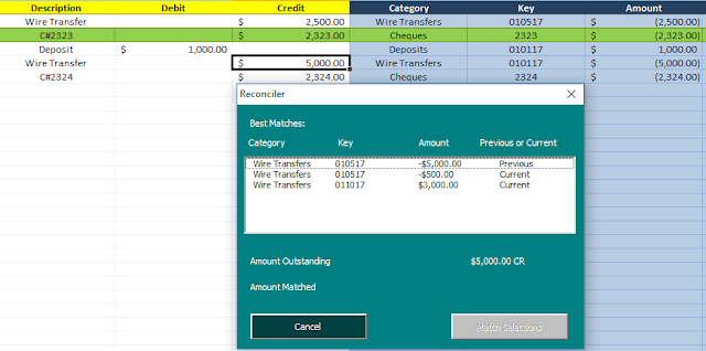
Alternative, you you can select a line item that has a status of O/S and click CTRL+SHIFT+X which will bring up the Reconciler window which will show you potential matches for the item you are looking to reconcile.
In the above example I pressed the shortcut keys while selecting the row with the $5,000 wire transfer. Since it is O/S it pulls up the Reconciler window. The Reconciler shows all the wire transfers from both the previous O/S tab as well as the Bank tab (in this example I was on the Book tab). Exact dollar matches show up at the top. Note the first result shows an amount of -$5,000 – the negative does not indicate a credit, it pulls the amount from the amount field which just shows the negative as being an outflow of cash. Because an outflow of cash on the bank is a debit, if I select the -$5,000 it will show $5,000 DR as being the amount matched, which is shown on the next screen:
Because the debits match the credits, the Match Selections button has turned green and can now be pressed. Doing so will enter an ‘X’ in the manual override field for these amounts. You will only be able to match the selections if the debits and credits match. You can select multiple items if they add up to the total outstanding.
Completing the Bank Reconciliation
Once all the bank and book data are entered and you have finished matching which items you can, go to the Reconciliation tab where there you will see three buttons on the right hand side:
The Reconcile button will generate the reconciliation and show you which items are outstanding. It will group the outstanding items by category – refer to the screenshot at the beginning of the post. If the adjusted balances match and the amounts reconcile to 0 then it will highlight that line in green, otherwise it will be in red to indicate a variance. The reconciliation date you will need to enter in the yellow highlighted cell.
The New Month data will clear all your existing data but before doing so will put your existing O/S items into the Previous OS Items tab so on your next month’s reconciliation they can be used to match new transactions.
For example, if cheque #1111 does not clear this month it will be moved to that tab. If on next month’s transactions there is a transaction on the bank for this cheque number the template will be able to reconcile it automatically. Nothing extra needs to be done to do this, as when looking for matches, both the bank and book tabs look at the Previous OS Items tab to clear any items from there as well.
Lastly, the Clear Data button will do just that – get rid of everything from every tab.
The template at the top has some sample data so you can test out and see how it works.
In VBA there is a custom DateDiff function that allows you to easily calculate the difference between dates – whether you want the difference to be in days, weeks, months, years, it is easier to accomplish this in VBA than through regular Excel formulas. I have piggy-backed off the DateDiff function to make a custom function in Excel that makes it easy to use as a formula in your spreadsheet.
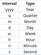
The custom function I have created is called datecalculation and consists of three arguments: start date, end date, and interval. The interval determines how the difference is calculated. The interval needs to be in quotations and use one of the following codes:
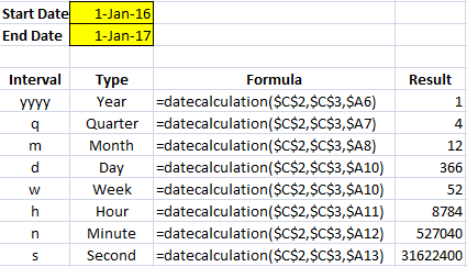
Below is an example of how the function work when computing the difference between January 1, 2016 (cell C2) and January 1, 2017 (cell C3). The interval codes are in column A.The result column is the date difference according to the selected interval.
To make this function work in your spreadsheet simply insert the following VBA code. If you are not sure how to do that, please refer to this post, specifically the section about inserting VBA code.
————————————————————————————————————————
Function datecalculation(date1 As Date, date2 As Date, interval As String)
This template allows you to create a customized letter – be it a cover letter or any other kind of letter from a pre-defined list of sentences and paragraphs that can also utilize variables. In order to accomplish this you will first have to setup the sentences, paragraphs, and variables you will want to use. But once you have done so you can easily reuse them going forward.
Setting Up Variables and Paragraphs
In my template I have two sections – one for variables, and one for paragraphs. In the variables section you can setup variables that can be used in your content. These will be values that will likely change from one letter to the next. In my example I have a % sign in front of the variable name. The purpose for this is to make it easier to accurately identify where a variable has been used. However you don’t need to use it, but you would want to ensure your variable name is unique and not a word that you might use in your content that you don’t intend to use as a variable.
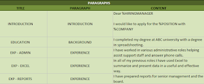
In the paragraphs section here you can setup sentences or entire paragraphs that you would potentially like to add to your letter. The title is just a way to identify the content, the paragraph is which paragraph the content relates to. For example, I have multiple titles that relate to the paragraph called experience.
This means that if I add all of these items, they will be stitched together to form only one paragraph. This is just to help organize my paragraphs to make sure I don’t have a paragraph for each item I want to add. You may not have enough to write a paragraph about each skill set you have, but instead you may want to add it on to a paragraph that relates to the content.
If I look at the title labeled ‘Introduction’ this has a related paragraph by the same name. There are no other items that relate to the introduction paragraph. So this means if I add the Introduction, it will be an entire paragraph on its own, and no other items I add will be added to it. The Introduction also has all three variables I setup – %HIRINGMANAGER, %POSITION, and %COMPANY. These are all variables that you would expect to change from one cover letter to the next. I can certainly use more variables and put them into other content but in this example I only did it in the Introduction.
If you need to add more rows you certainly can do that, as well as changing the existing content, titles, and related paragraphs. If you want to add lines within a cell, all you have to do is when you are editing in the cell click ALT+Enter and you will create an additional line of text within that cell. This will allow you to help space out your descriptions as you wish.
Updating Variables
Once your paragraphs and variables are setup, click on the Create Letter button. You will first be prompted to enter values for your variables. Here I will update the name of the hiring manager I’m applying to, the name of the company, and position.
Once done, click Update Variables.
Finalizing the Letter
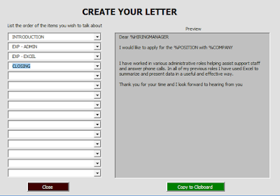
Next, you can select the content you wish to add to your letter. The titles will appear in the drop down boxes. Go from top to bottom. As you select an item it will be added to your letter.
When I add Introduction my variables are now updated to reflect what I entered at the earlier screen. You can also edit the letter in the preview box.
However should you make any changes to the drop downs your edits will be gone. So make sure to do edits only after you’ve selected all the content you wish to use.
Once you are done, click on the Copy to Clipboard button and you can now paste it into a word processing document, email, or wherever you like.
This template is designed to allow you to easily track and manager your expenses using budgets and copying transactions downloaded from your bank or credit card statement.
Once you have a download of your transactions from your statement, copy the data into the Import tab. The transaction dates into column A, the description from your statement in column C, and the amount in column D. Important to note that expenses should be positive (refunds negative), as should income. For payments/transfers I will cover further down but it will be negative if it is an outflow from the account/payment source or positive if an inflow. The source of your transactions will be selected in cell G2.
The suggested vendor column will autofill once it finds vendors matching the description you copied in column C. If not, you will want to setup the vendors using the setup button on the right of the page and click on manage vendors from where you can add, modify, and delete vendors. Once vendors are setup and all the suggested vendors are filled, click on the next button which is to Apply Names. This will fill the vendor column. After this is done you are ready to click on Copy Expenses. This will now move your transactions into the All Transactions tab. We focus on this tab next to go over how to manually enter transactions.
MANUALLY ENTERING TRANSACTIONS
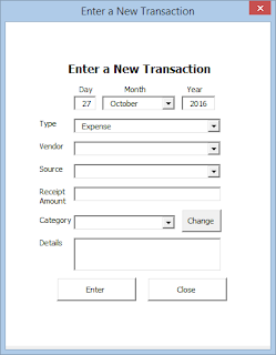
You can manually enter transactions from the All Transactions tab by clicking the New Expense button at the top (or CTR:+SHIFT+T as the shortcut key is noted in each of the buttons up top).
MODIFY TRANSACTIONS AND ALLOCATIONS
You can also modify existing transactions by clicking on the Modify Transaction button on the same tab which is the same screen as the new expense screen (see below) except filled out with the selected transaction’s details.
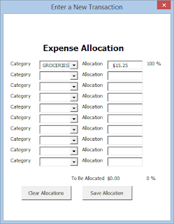
Additionally, you can change the allocation. When setting up a vendor you assign a default category. However in this template you can break out a line item into as many as ten different cost categories. For example, if you go to a department store it may not be as simple as saying all those expenses relate to groceries, clothing, baby items, electronics, or whatever else is sold there. You could have all those cost categories and more in one receipt. This is where you can break out that detail, by clicking on the Change button next to the category drop down.
ACCOUNT TRANSFERS/CREDIT CARD PAYMENTS
Payments from one account to another are not an expense and may not be important enough for you to track. However, for the sake of completeness and making sure all your transactions are accounted for and balances reconciled, this can be accomplished here by setting up a vendor equal to the name of another payment source. In this template if you make a payment from one payment source to another it is recognized as a transfer rather than an expense (in the manual entry screen you can also specify transfer rather than expense). If the source of your payment is the bank and your vendor is your credit card (e.g. you are paying your credit card from your bank account) then on your bank account this amount should be negative and on the credit card it will be a positive. Transfers should add up to 0 every month unless you are missing one side of the entry. You can also manually enter transfers from the AllTransactions tab. Again, transfers are not necessary but helpful for the sake of reconciling to make sure all balances match.
ACCOUNT BALANCES
The Balances tab is used for reconciliation purposes to make sure the balance on your statement at the end of the month matches the balance here. It will reconcile according to the statement month and year rather than just looking at the calendar month and year. This will allow you to more easily reconcile to a specific statement. In row 17 you will want to enter any opening balance you have from these accounts.
BUDGET CATEGORIES
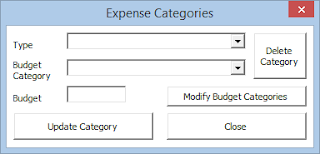
You can create budgets and also break them into multiple categories. By default I have setup my categories into whether the expenses are essential, discretionary, or irregular. However you can change these from the setup button (from the All Transactions or Import tabs), selecting Manage Expense Categories, and then selecting Manage Budget Categories.
From the Managing Expense Categories section you can create, modify, and delete budgets as well as change monthly amounts.
CASH FLOW AND PER DOLLAR SPENDING
These tabs show spending based on the budgets created and arranged in accordance with the different budget categories.
SUMMARY
Lastly, the summary tab provides a summary of the expenses. In row 1 you can specify the month, year, and budget category you wish to review. The bar graphs below show in red how much an expense is over budget, and if there is dark green that indicates the budget has been partially used and the dollar amount specifies how much has been used with the light green portion what is remaining
Further down below the graph you will see a summary of the largest expense items, as well as top items by category where you will be able to select multiple expense categories to review at once. Alternatively, you could also go to the All Transactions tab and filter the data from there to view what made up an expense category. NOTE ABOUT CUSTOM FUNCTIONS There are multiple custom functions in this template and occasionally they might get stuck – show an error instead of the calculated value. To correct this just hit ctrl+alt+F9 if you notice error values as this should fix the issue.
This function works as if you were doing multiple lookup statements in one formula. The example I’m going to use is if you wanted to look at your credit card statement and from the description determine what vendor it is.
For this function to work I need to create a named range of all the values (e.g. possible vendors) I want to cycle through to compare the string (e.g. credit card data) against. The named range needs to be called LookupList. Below you will see the LookupList I created. (For more on named ranges, see this post)
I’ve added a header but that is not necessary. As long as the list is a named range called LookupList. The adjacent column is the value that will be returned if the value in the LookupList is found. You need to ensure this column is also filled in or else the result of the formula will be blank, regardless if there is a match.
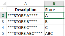
When I run the custom function, the function will cycle through the LookupList from top to bottom to see if one of those values is in the cell I am using the formula on and if so, return the related result. For that reason, the LookupList also needs to be in descending order, to avoid a premature match (e.g. finding Store A before the function finds Store ABC)
Column A is an example of data from a credit card or other source that may have various characters before and after what you are looking for. You could use the MID function to extract that data but that will only work if that data is consistently arranged the same way. It might be, but using this function it won’t matter and it will just look if any of the values in the LookupList are contained in the string, regardless any other characters before and after.
Column B is the MatchThis function. And since the LookupList is already defined the only argument is the data that you want to look at, which in this case is column A. In column B2 the formula is simply =matchthis(A2). Because it matches Store A, it returns the value A (from the results column).
Below is the code for this function:
————————————————————————————————————————————–
Function MatchThis(matchcell As Range)
Application.Volatile
Application.Calculate
Dim LookupList As Range
Dim c As Range
‘Identify the range of cells you want to compare against. The lookuplist is what will be compared against and the column to the right of it will be the output
Set LookupList = Range(“LookupList”)
‘Go through each of the cells looking for the criteria in cell c, and if it matches, pull the value from the next column
If you’re looking for a way to manage your employee expense reports and don’t want to shell out hundreds of dollars every month, then this expense report template could be a great option for you. You can set up rules and flags for categories and it will keep track of when and who a report was approved be.
Benefits of using this expense report template
The expense report template is designed to help with the following:
Unlike online reporting solutions, you have all the data and can store and save it as you wish.
Complete customization. Setup multiple approvers, categories, and flags as you need.
Make it easy for employees to enter expenses across multiple categories and branches
Allow management to easily change and setup desired limits for expenses
Bringing problem items to the attention of managers to force them to acknowledge and allow them to comment on individual issues.
An approval process that stamps the date, time and user ID of the employee who has reviewed the report and the manager who approved it.
Integration with the ribbon so buttons are readily available in the tab.
Setup limits for expenses
Let’s move over to the SETUP tab. This will show you the customization you can do with this report.
Under the expense categories section I can specify the dollar limit per category, the GL code, as well as if it is per attendee (PerAtt). The limit is at what amount the expense gets flagged. It won’t prevent the user from completing the report, but the limit instead acts as a way to flag expenses over the limit.
For example, in my table below if someone made a claim for $3,000 for air travel, it would get flagged for the manager to review.
In the case of meals, this is a moving target since it is largely dependent on the number of people at a given meal. If it is a company even with dozens of people then a limit of $50 or $100 will not be terribly useful. This is where the PerAtt column comes into play. For meals at $50 and an “X” marked in the PerAtt column, the $50 limit will be multiplied by the number of attendees indicated on the expense report (the data tab has this information). This will allow the limit to grow with the number of people in attendance.
The GL code column is for accounting purposes as to which account it should be booked to.
Other setup options
In the next section of the setup tab it relates to branches and what GL suffix is to be added if necessary. If no branches are used this can be left blank. The accounting password is what will need to be entered when the accounting button is pressed at the data tab which will unlock all the tabs including setup. Also, there is a section for a list of employees and their approvers and the approver passwords.
If you need to set up more approvers or sections, make sure to insert a row above the last entry to ensure that formulas remain intact.
The last section in the setup relates to the GL coding for which account to credit as well as the tax account.
Using the data tab
The DATA tab is where all the data entry goes. I have filled out some expenses as below. Since both of them are over my pre-defined limits, they will both be flagged.
Once the file is sent to the manager for review, he will press on the Manager Review button which will prompt for a password. If correctly entered, the Manager tab will show and it will show the following items as being flagged:
The information is pulled from the data tab and under the reviewable reason it explains why it has been flagged. There is also space for the manager to put their comments regarding the items so that once the report is sent to accounting for processing accounting will see any comments by the manager to confirm they have acknowledged and approved the expenses.
Finally, the accounting tab prepares the GL entry. This is triggered once the accounting button is clicked and password is entered
When creating a complex formula sometimes you use multiple cells to get to a desired result. Then at the end you may want to join all those cells into one large formula. You can do this by copying formulas to replace the cell references but it’s not as easy as it should be.
The macro below does exactly that – it will replace the cell references with the formula in the referenced cell. For example, in cell A1 I have a simple formula of =5*5.
In cell A2 the formula is =A1+10.
What I do next is to select cell A1 and run the macro. It will look in the spreadsheet to see everywhere that cell A1 is referenced and replace it with the formula in A1. Below is the result in cell A2 after the macro has been run:
You’ll notice I added parentheses to make sure that the result would not get altered – not applicable in this example since order of operations would ensure the calculation is correct but in a more complex example it might not be the case.
Below is the code for this macro:
Sub copyformula()
Dim whattocopy As String Dim whattoreplace As String