vba Archives - Page 2 of 4

How to Customize the Excel Ribbon Using the Custom UI Editor

July 27, 2021

by howtoexcel with No Comment macros ribbon vba

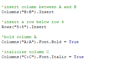
In a previous post, I covered how you can customize the Excel ribbon in what was a pretty manual process. The good news is there is a much easier way to make changes to the ribbon using the Custom UI Editor. Below, I’ll cover how you can add and remove both tabs and groups, how to add buttons, and how to even use your own images. The first thing you’ll want to do is to download the Custom UI Editor. There’s not a definitive place you can always find this tool at so your best bet is to do a Google search.

How the Custom UI Editor works

Once you have downloaded the Custom UI Editor, you can get to work and begin to customize the Excel ribbon. Unlike just a simple customization, when you modify the ribbon using the Custom UI Editor, you are making changes to the Excel file itself. That means when you send the file to someone, they will see the changes you have made. With just a ribbon customization, those changes only apply to your computer. But these changes will be saved within the file. The Custom UI Editor goes through the cumbersome process of attaching the XML code to the Excel file and makes it a lot easier to make changes to the ribbon.

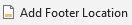
When you first open the file, you’ll see a blank canvas such as this:

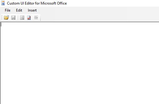
Start with clicking on the Folder icon to load up the Excel file that you want to modify. Any Excel file will do. Next, go to the Insert menu and click on Office 2010 Custom UI Part:

This will create the xml file for Office 2010 and newer versions of the ribbon. If you want to ensure these ribbon modifications also work on Office 2007, then you will want to also insert the file for Office 2007 Custom UI Part. If the file isn’t going to be used on an older version of Excel, this isn’t necessary, but it also doesn’t require much additional effort.

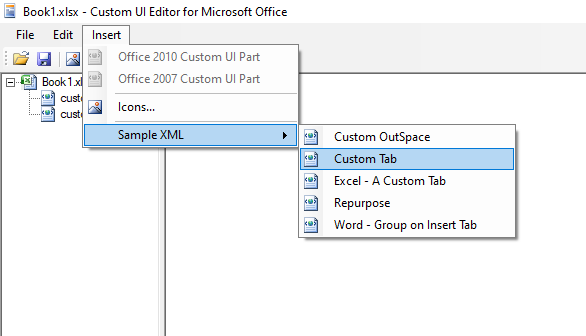
The Custom UI Editor includes some sample code within it that you can automatically load so that you don’t have to start from scratch. With one of the xml files selected, let’s go back to the Insert menu, and this time click on Sample XML and Custom Tab.

Inserting sample XML from the Custom UI Editor.

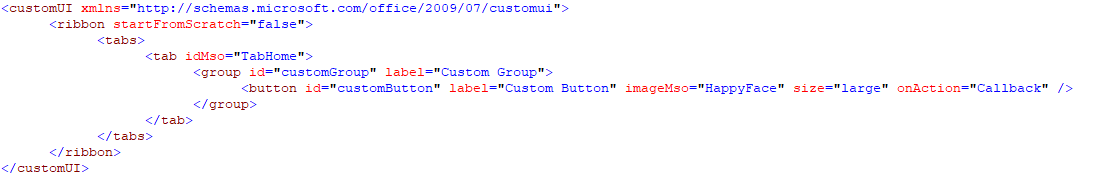
This will insert some xml to get you started:

The Custom Tab XML code is loaded into the Custom UI Editor.

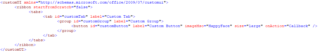
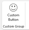
What the code has done is created a tab called Custom Tab and within that, created a Custom Group. Lastly, it has also added a button called Custom Button, which is a large size and uses a HappyFace icon that is built-in within Excel. Here’s what that looks like in the actual Excel file:

Custom button using the Happy Face icon.

The one thing that’s left to do is to link the button to some VBA code so that it does something when you click on it. I’ll cover that towards the end of this post.

If you wanted to run this same xml code for the older version of Excel (2007), then everything would work the same except for the very first line. Instead of this:

<customUI xmlns=”http://schemas.microsoft.com/office/2009/07/customui”>

You would use this:

<customUI xmlns=”http://schemas.microsoft.com/office/2006/01/customui”>

All you need to do is change 2009/07 to 2006/01.

To check that your code is correct, you can click on the red checkmark icon at the top:

And if you get this message:

Custom UI message saying the XML is well formed.

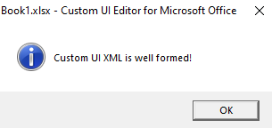
Then your code is good to go and doesn’t contain any (obvious) errors.

Adding a custom button to the Home tab

Using the above example, you can customize the Excel ribbon to create a group and custom buttons inside of a new tab. However, I prefer simply adding any custom buttons on the Home tab to make them easy to find. Unless you have many buttons and macros, you probably don’t need to put them on an entirely separate tab of their own.

If you don’t want to create a new tab and just want to put your buttons in an existing tab, then you can use the following code to put them on the Home tab:

<tab idMso=”TabHome”>

When you use a reference of ‘Mso’ that means it is an existing Microsoft tab/group/image. You need to refer to the correct name (see further down for a list of groups and tabs) and then you can put your custom group or button in that tab rather than creating a new one. Here’s what the full code would look like by changing this one reference from the above example:

Custom UI Editor showing button group created within the Home tab.

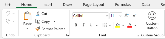
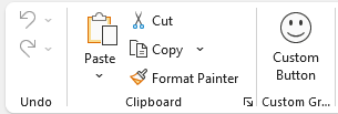
In Excel, I still have my custom group, but now it isn’t on its own tab. Instead, it goes to the end of the tab:

Custom group showing at the end of the Home tab.

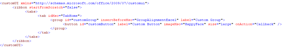
If it’s too far to the end what you can do is insert it before a certain group. Let’s say I want to put it just before the Alignment group. Then I just need to adjust the code slightly to add the insertBeforeMso (this is case-sensitive) attribute for the group tag:

<group id=”customGroup” insertBeforeMso=”GroupAlignmentExcel” label=”Custom Group”>

This is how the full code looks:

Custom UI Editor with custom group inserted before the Alignment group.

And now my custom tab shows up a lot earlier in the home tab:

Custom group and button showing on the home tab after the Font group.

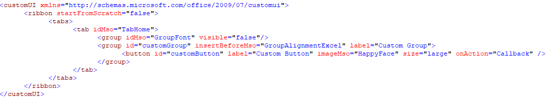
Another thing I can do is also remove some groups. If I don’t want the font group, I can add the following line of code in the Custom UI Editor:

<group idMso=”GroupFont” visible=”false”/>

Here is the updated code:

Custom UI Editor that shows line removing the Font group.

And here’s what the ribbon looks like:

You could make all the Microsoft tabs and groups invisible if you wanted to and can control where you custom group goes. The key is knowing the correct names.

Names of the Microsoft tabs and groups

Here is a list of the Microsoft tabs and the reference you will want to use when modifying the ribbon:

Tab Name	RibbonX Referenece
Home	TabHome
Insert	TabInsert
Draw	TabDrawInk
Page Layout	TabPageLayoutExcel
Formulas	TabFormulas
Data	TabData
Review	TabReview
View	TabView
Developer	TabDeveloper

Here are the main groups from the Home tab:

Group Name	RibbonX Reference
Font	GroupFont
Alignment	GroupAlignmentExcel
Number	GroupNumber
Styles	GroupStyles
Cells	GroupCells
Editing	GroupEditingExcel
Clipboard	GroupClipboard
Undo	GroupUndo

There are more groups (from other tabs) but for this purpose, I just included the most common ones.

Adding an image to a button

If you want to use an existing Microsoft image for your button, then you can view the imageMso gallery here. Once you find the image you want to use, just put that in place of the HappyFace image in the earlier code.

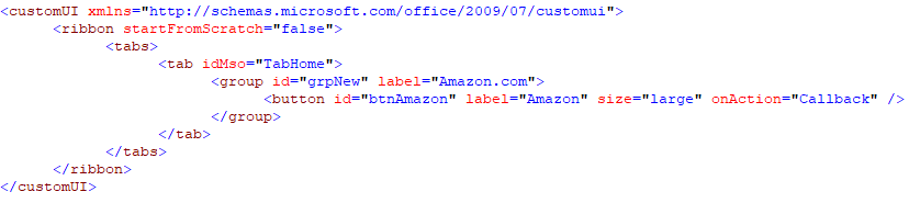
However, suppose you want to make a custom image. I’m going to create one using the Amazon logo to create a button that will open my browser to the Amazon.com website.

For starters, I need to get an image. For large ribbon buttons, you want to aim for a size of 32 x 32 and for smaller images, 16 x 16. As long as it’s a square image, however, you should be okay. Wide images will stretch and won’t look as good. This is the image I’m going to use:

I’m going to use just a simple code for creating the button, which looks as follows:

Custom UI Editor showing code for the Amazon button.

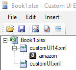
I haven’t associated an image to this button yet. To do that, I’m going to click on the xml file and go back to the Insert menu. This time, I’m going to select Icons. This will open up launch a dialog box where I can now select the image I want to use from my computer. Once I’ve selected it, it now shows up underneath my xml file:

Image file showing attached to the xml file.

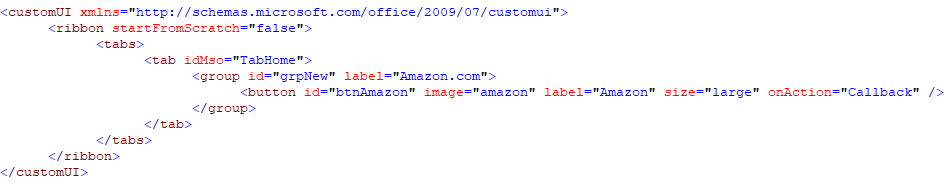
I can right-click on the name ‘amazon’ to change the id to something else. Whatever if it is, that’s what I need to reference in my xml code. Since it’s not a Microsoft image, I just add the following attribute:

image=”amazon”

And here is my full code:

Custom UI Editor showing the code referencing the custom image.

If I open up Excel, this is what my custom button looks like:

But right now, my button doesn’t do anything. That leads us to the last section on how to customize the Excel ribbon: callbacks.

Setting up callback macros

A callback tells the button which code to run. So that means you need some VBA code to begin with, otherwise, the button isn’t going to do anything. I’m going to create a simple macro that will just open the Amazon.com website:

Sub Amazon()
ActiveWorkbook.FollowHyperlink (“https://www.amazon.com”)
End Sub

The callback function itself can be generated from the Custom UI Editor. If I click on the icon next to the checkmark that looks like a block of code:

The application will produce the VBA code I need to put into my Excel file:

Callback generated from the Custom UI Editor.

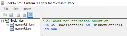
I’m going to copy and paste that back into VBA. However, I need to add a line in between as that code only sets up the macro, it doesn’t do anything yet. I need to reference the macro I created earlier. The full callback macro looks as follows:

‘Callback for btnAmazon onAction
Sub Callback(control As IRibbonControl)
Amazon
End Sub

Now when the button is pressed, the ‘Amazon’ macro will run, which opens the Amazon.com website. You can create a custom button for each macro you want to run and assign an image to each one. All you need to do is to use the callback macro to link the button to the code you want to run.

If you liked this post on How to Customize the Excel Ribbon Using the Custom UI Editor, please give this site a like on Facebook and also be sure to check out some of the many templates that we have available for download. You can also follow us on Twitter and YouTube.

Excel Automation: 10 Tasks You Can Automate Today!

November 29, 2020

by howtoexcel with No Comment functions intermediate macros tips & tricks vba

Spreadsheets can allow you to analyze data and create reports efficiently. But sometimes the tasks that are involved can be difficult or appear to be time-consuming. The good news is that there’s a lot of automation you can achieve in Excel, and it isn’t always necessary to know how to code in order to do so. Below, I’ll show you 10 types of tasks that you can automate in Excel either on your own or with our help.

1. Cleaning and parsing data

One of the more challenging things in Excel is when you’re dealing with a dataset that may not be easy to manipulate. For instance, if you’ve got text mixed in with numbers or dates that aren’t in the right format, Excel may not interpret or recognize the data properly. But there are many formulas that can help you with that. Rather than manually fixing the data, you can use functions like TRIM, CLEAN, LEFT, MID, and RIGHT to extract what you need while also getting rid of extra, unnecessary spaces and other characters.

If you’re looking for more of a walkthrough of the process, there’s a detailed explanation in this post of how to parse data.

Through the use of formulas, you can save hours that you might otherwise spend trying to clean up your spreadsheet. And the best part is that once you’ve set it up, you can re-use the formulas as you add more data. You don’t need to use macros or complicated coding to clean up; a well-structured template can be enough to do the job for you.

2. Creating simple reports

One of the best features of using Excel is that once you’ve entered data into a spreadsheet, it’s even easier to create a report from it. One example is through the use of a pivot table, where through just a few clicks you can easily summarize your data and split it along different categories. Slicers can make filtering and summarizing data even easier in pivot tables, especially for users who aren’t very familiar with Excel. Forget any manual work here; just a few clicks and you’ve got a report that can quickly summarize information in a table for you!

Alternatively, you can also insert charts easily and Excel will try and select the best one based on your data set. There’s also lots of formatting you can apply to charts so that they have the look and feel that you’re after. And once you’ve got a look that works, you can re-use it over and over again.

3. Creating dynamic dashboards

Dashboards are incredibly popular but they can be complex to set up. Then there’s also the challenge of updating it and making sure the data is up-to-date. It can easily take you hours every time to make sure the information is accurate.

However, in this post, I show you how to create a dynamic dashboard that not only won’t take you hours but that will automatically update as you add data to it. And then, you end up with a report that looks great to send to management to easily review and update.

4. Routine data entry

One of the biggest headaches people can face when using spreadsheets is when they hard-code calculations. A hard-coded calculation is where you don’t reference any cells and just put the result in the cell; it can make it nearly impossible to decipher how that number was calculated (especially if you’re not the person who entered the value). If you go to re-calculate it or update it, you could spend a lot of time just trying to figure out the calculation.

However, by using a formula, there’s no ambiguity as to how a value was calculated. Not only does that save you the time of entering in data but it also makes it easy to correct and update the figure. Ideally, you should minimize the number of places you’re manually entering data into. By doing that, you’ll have a much more robust template where your inputs are kept to a minimum which will eliminate the need for a lot of data entry and your other calculated fields will update automatically. This type of automation doesn’t require complex coding and just needs an Excel spreadsheet to be carefully constructed so that it is efficient and makes the most of formulas.

5. Conditional formatting

Oftentimes you’ll want to color-code your data to highlight things you should be paying attention to. If you’ve got an aged accounts receivable schedule, it is useful to highlight which accounts are more than 90 days overdue. You could manually filter the data and highlight all the cells or rows in red that are overdue, but you can just use conditional formatting to do that for you.

Through conditional formatting, you can create rules to determine when a cell or row should be highlighted in red, when you may want it to be in yellow, or when you may just want to hide the text so that you can easily skip over it. For example, hiding zero values can make it easy to focus on more important numbers.

You can apply many different formatting rules and can even put in a hierarchy to determine if you want to keep applying formatting rules or whether you want to stop if a specific criteria is met. Conditional formatting can be complex but it can be a huge time-saver by allowing you to focus on just the items that are important to you. And once you’ve set up the rules, you don’t need to worry about making changes every time you add new data.

Check out this post to learn about conditional formatting and how you can apply it to your spreadsheet.

6. Updating other workbooks and sheets

If you use multiple workbooks, then another area where you can avoid re-entering data is by linking both workbooks. There are numerous ways that you can do this. One approach involves just linking directly to another worksheet where data will automatically pull from another table.

You can also use the INDIRECT function to reference another worksheet or workbook. Just like with a template, once you set up these formulas and connections, they are there to stay and you can avoid having to manually make changes by yourself.

7. Audit tracking by logging changes

One of the neat features of many Office products is they allow you to track changes that are made. This is normally when you share a workbook with other users. However, through the use of macros, you can have a separate sheet that can tell you which values were changed, when, and by who.

Rather than manually noting these changes or relying on people to make the updates themselves, it doesn’t take much effort through a macro to create a log of what’s been changed.

8. Generating PDFs

One thing many advanced Excel users like to do is to use automation to export reports into PDFs. While there is a way to print to PDF, and it’s particularly easy on the newer versions of Excel, it can be a time-consuming process especially when you need to print out multiple sheets. Here again, with a simple macro, you can auto-generate PDFs and save them in a predefined folder all with the click of a button.

9. Sending emails

Another feature many users like is the ability to use automation to send out emails right from Excel. Through the use of macros, this is also possible. You can create a macro that will enter in the email of the recipient, attach a file, enter the body of the message, and even send the email itself. This can be even set up on a large scale, such as sending out invoices to dozens or hundreds of customers, a process that could easily save you hours worth of work.

10. Just about anything else with VBA

The power of programming in Excel can unlock many different possibilities with what you can automate. Whether it’s using automation to help import data and then manipulating it, creating custom reports, or following a series of complicated steps, there are many tasks in Excel that can be expedited with a few clicks of a button. As long as there’s some logic to the process that you can break into steps, then you can also build that into the code and automate it.

Don’t know where to start? Contact us!

There is significant potential in Excel but not everyone knows how to use automation to make the most of it and to make a spreadsheet as efficient as it can be. You can contact us if you have a certain Excel issue that you need help with or if one of the tasks above has perked your interest and you’d like to learn more. We can help create solutions for you that work efficiently and that can save you many hours, perhaps even days every month.

If you liked this post on 10 Tasks You Can Automate Today, please give this site a like on Facebook and also be sure to check out some of the many templates that we have available for download. You can also follow us on Twitter and YouTube.

Convert a Summary Table in Excel Into a Pivot Table

June 6, 2020

by howtoexcel with No Comment advanced data entry macros pivot table vba

Often times, when you download a data table from somewhere it’s not in the format you need it to be. Tables are often in a summary format where you have months going down and years going across, or vice versa. It’s the end result of what you want a pivot table to look like, but you can’t easily turn that into a pivot table itself. Below, I’ll show you how to turn a summary table in Excel that looks like this:

Into this:

This format is much more Excel-friendly and one that you can easily convert into a pivot table.

Converting the table

The data I’m using is the same one that I used in an earlier post that went over transposing data. Transposing data, unfortunately, isn’t enough to make data workable if you want to convert it into a pivot table. You’ll want data to be in a tabular format so that there’s a header for the month, year, and value.

You could manually transpose one year at a time and copy the data one by one. But of course, that isn’t optimal at all. The good news is I’ve got a macro that can help you flip that data in one click. It will go through the painstaking process of reorganizing the data for you.

Here’s the code for the macro. You can just put it into a module (I’ll leave a template to download below if you aren’t comfortable doing this step yourself):

Sub flipdata()

Dim cl, nxtcl As Range
Dim lastcol, lastrow, firstcol, firstrow As Integer


'get total number of rows and columns in range
lastcol = Selection.End(xlToRight).Column
lastrow = Selection.End(xlDown).Row

'get first column and row
firstcol = Selection.Column
firstrow = Selection.Row

'assign output starting point
Set nxtcl = Cells(lastrow + 2, firstcol)

nxtcl = "Header 1"
nxtcl.Offset(0, 1) = "Header 2"
nxtcl.Offset(0, 2) = "Value"

Set nxtcl = nxtcl.Offset(1, 0)


'cycle through data

For yr = (firstrow + 1) To lastrow

    For mth = (firstcol + 1) To lastcol

        nxtcl = Cells(firstrow, mth)
        nxtcl.Offset(0, 1) = Cells(yr, firstcol)
        nxtcl.Offset(0, 2) = Cells(yr, mth)
        Set nxtcl = nxtcl.Offset(1, 0)

    Next mth

Next yr

End Sub

It will output the data a couple of rows below where your data ends. It’s important to select the entire range of data before running the macro since it will go through the range that you’ve selected, nothing else. And if there’s data below your selection, it will overwrite that.

After you’ve selected the data, then you run the macro. In my template, I’ve got a button that you can press that will do the job for you and then you’ll get something that looks like this:

Once in this format, you can easily create a pivot table:

If you’d like to download the file that contains the macro, it’s available here.

If you liked this post on how to convert a summary table in Excel into a pivot table, please give this site a like on Facebook and also be sure to check out some of the many templates that we have available for download. You can also follow us on Twitter and YouTube.

How to Make a Countdown Timer in Excel

May 23, 2020

by howtoexcel with No Comment dates macros template vba

A countdown timer can help you track how much time there’s left to do a task or until a deadline comes due. Below, I’ll show you how you can make a countdown timer in Excel that can track days, hours, minutes, and seconds. In order to make it work, we’ll need to use some VBA code, but it won’t be much. And if all else fails, you can just download my free template at the end of the post and repurpose it for your needs.

Let’s get right into it and start with the first step:

Calculating the difference in days,

To calculate the difference between two dates is easy, as all you’re doing is subtracting the current date and time from when you’re counting down to.

The start date is just going to be today, right this very second. And Excel has a convenient function just for that, called NOW. It doesn’t require any arguments and all you need to do is enter the following formula:

=NOW()

Entering the date and time you’re counting down to is a bit trickier. As long as you enter it correctly, then calculating the differences will be a breeze. However, this may involve a little bit of trial and error since it’ll depend on how your regional settings are setup. For the countdown date, I’m going to set it to the end of the year. Let’s say 11:00 PM on New Year’s Eve. Here’s how I input that into my spreadsheet:

2020-12-11 11:00 PM

The key things to remember here are that there should be a space between the time and the AM/PM indicator (if you use it) and there should be two spaces between the date and the time. Then, it’s just a matter of whether you’ve got the right order of date, month, and year. This is where you may need to do some testing on your end to ensure you’ve got the correct order.

Now that the dates are set up, we can calculate the difference in days. To do this, we can just calculate the difference and use the ROUNDDOWN function to ensure we aren’t adding partial days:

There are 222 days left until the end of the year. By using the NOW function, the formula will automatically update and tomorrow the days remaining will change to 221, and so on. If your output’s looking a little different, make sure to check the formatting and that it’s set to days.

Calculating the difference in hours, minutes, and seconds

There’s not a whole lot of complexity when it comes to calculating the difference in hours, minutes, or seconds. We’re still subtracting the current date from the deadline. The only difference is that now we’re just going to change the formatting. If I do a simple subtraction, I end up with a fraction, which isn’t really usable in its current format:

Counting down the hours, minutes, and seconds left.

The trick here is to change the format of this cell so that it shows me hours, minutes, and seconds. And that’s an easy fix. If I just click on cell C10 and click CTRL+1, this will get me to the Format Cells menu. In here, I’ll want to select a Custom format so that the cells just shows hours, minutes ,and seconds:

Here’s what the countdown timer looks like after the format changes:

It’s important to include a date in the calculation even though we’re just doing a difference between hours, minutes, and seconds. Otherwise, the formula wouldn’t correctly calculate in all situations, such as when the deadline hour is earlier than our current hour.

Putting it all together

Now that all the calculations are entered in, now it’s just a matter of formatting the data. We can create a countdown clock that separates days remaining, from hours, minutes, and seconds remaining.

One cell can have the difference in days, while another will have the difference in hours, minutes, and seconds. This goes back to just modifying the formatting and applying a custom format. Here’s how mine looks:

Although we’ve gotten to this point, the challenge is that this countdown timer still doesn’t update on its own. Unless you want to click on the delete button all the time, the countdown isn’t going to move unless there’s something to trigger a calculation in Excel. That’s why we’re going to need to add a macro to help us do that, which bring us to the important last step of this process:

Adding a macro to refresh every second

We need a macro to update the file. Whether it’s every second, every five seconds, it’s up to you. While the countdown timer will update when someone enters data or does something in Excel, that’s not much of a countdown. This is where VBA can help us. If you’re not familiar with VBA, don’t worry, you can just follow the steps below and copy the code.

To get into VBA, click on ALT+F11. From the menu. Once you’re there, click on the Insert button on the menu and select Module:

Over to the right, you’ll see some blank space where you can enter in some code. Copy and paste the following there:

Sub RunTimer()

    If Range("C10") <> 0 Then
        Interval = Now + TimeValue("00:00:01")
        Application.Calculate
        Application.OnTime Interval, "RunTimer"

    End If
End Sub

One thing you may to change is the reference I made to cell C10. Change that to where you have your countdown timer. As long as there’s a value in the cell, the macro will continue running. All it does is check if there’s a value there, and if there is, it updates the worksheet every second. And by doing that calculation, your countdown timer will update even if you’re not making any changes to the spreadsheet.

You can also change the interval which currently updates every second, as noted by the 00:00:01. You can change this to five seconds, 10 seconds, however often you want it to update.

But there still needs to be something that triggers the macro to start running. You can assign a button or shortcut key to do that.

However, in this example I’ll activate it when the sheet is selected. Inside VBA, you should see a list of worksheets. Double-click on the one that contains your countdown timer:

You’ll again see blank space to the right where you can enter code. And you’ll also see a couple of drop-downs near the top that you’ll want to look for. By default, the first one should say (General). Change this to Worksheet:

Next, change the other drop-down which will probably say SelectionChange. Change it to Activate. Then you should see something like this:

Selecting the worksheet activate event in VBA.

Copy the following code into there to call the macro we created above:

RunTimer

Now when you switch to another worksheet and come back to the current one you’ll notice your countdown timer is updating on its own. If you want it to stop it, just clear the cell that has the timer. Otherwise, the macro will continue running every second.

The Countdown Timer Template

If you’d rather just use a template, then you can download one that I’ve made here. You don’t have to worry about macros and instead you just need to enter the end time; the time that you’re counting down towards.

I’ve also got a start/stop button that you can toggle to get the countdown timer going and that will pause it:

You can move the button as well as the time your counting down to onto another sheet if you don’t want someone altering it. If you have any questions or comments about this template, please send me an email at [email protected]

If you liked this post on how to make a countdown timer in Excel, please give this site a like on Facebook and also be sure to check out some of the many templates that we have available for download. You can also follow us on Twitter and YouTube.

This Macro Converts Your QuickBooks Export Into a Table-Friendly Format

December 22, 2019

by howtoexcel with No Comment accounting add-ins formatting macros template vba

QuickBooks does a good job when it comes to recording sales and doing day-to-day accounting tasks. You may be content with the reports that come out of QuickBooks, too. But if you’re looking for some more in-depth analysis to do of your own or to make your own reports, you’re likely going to want to move that data into Excel. And, unfortunately, the QuickBooks export into Excel can be less than optimal.

With many spaces, subtotals, and a non-tabular format, it’s not a very practical output to use in Excel. If you want to run a pivot table and do some serious analysis in Excel, you first have to clean up the data before being able to use it, and that can be a very tedious and tiresome process.

For example, this is what your QuickBooks report might look like when you’re pulling a simple summary of your customer sales:

There are a lot of things that need to be adjusted for this report to be useable in Excel, including getting rid of the blank spaces and ensuring that the customer information is repeated in the first column, as opposed to just in the first line and in the last line’s total. From afar, it’s a bit of a painful process to have to go in and clean this up. And while it’s not impossible, it’s not going to be quick, either.

That’s where a macro can help you make the task much quicker and it will save you a lot of time if you have to go through these steps often. Click the button on the ribbon and your data will convert into a more table-friendly format! Here’s how it works:

Using the macro to fix the QuickBooks export

Before running the macro, you’ll need to specify the columns where your customer names and dates are:

Then, run the Covert Data button:

Downloading the file

The free version of the QuickBooks macro will allow you to run the conversion if it doesn’t go past 100 rows. However, if you decide to purchase the full version please ensure that the macro and file works as expected. There’s no guarantee the QuickBooks export hasn’t changed or won’t change in the future. If there are changes that need to be made to the macro, please feel free to contact me so that I can make the necessary adjustments. Whether you prefer the add-In or the actual Excel spreadsheet itself, both versions are available both here and in the paid version as well.

Here is the download link for the add-in as well as the Excel file. For the paid versions, please visit the product page.

If you have another program or software that you’d like a similar add-in for, I can help with that as well.

If you liked this post, please give this site a like on Facebook and also be sure to check out some of the many templates that we have available for download. You can also follow us on Twitter and YouTube.

How to Customize the Ribbon in Excel Using XML

June 12, 2019

by howtoexcel with No Comment advanced ribbon vba

If you want to customize the ribbon in Excel then you know simply changing doing it through the front end is only going to work on your computer. The customization isn’t technically saved within the file and it won’t move from one file to another unless you actually adjust the xml.

It’s by no means an easy process, but if you’re just looking to add a custom tab with some buttons for some macros that you have, I can show you a quick way to do that as painlessly as possible. It’s by no means comprehensive, but it’ll get the job done.

Step 1: Open your Excel file in a program like Winzip/7-Zip

If you right-click on your Excel file you should have an option that says Open Archive if you have a program like Winzip or 7-Zip installed. There, you should see something that looks like this:

These are the files and folders that are within the Excel file itself.

Step 2: Create a folder called customUI

Step 3: Open up notepad and paste the following into it:

<customUI xmlns="http://schemas.microsoft.com/office/2006/01/customui"> <ribbon startFromScratch="false"> <tabs> <tab idMso="TabHome"> <group id="myMacros" label="My Macros"> <button id="Macro1" label="Macro1" imageMso="HappyFace" size="large" onAction="cbMacro1" /> <button id="Macro2" label="Macro2" imageMso="TableDrawTable" size="large" onAction="cbMacro2" /> </group> </tab> </tabs> </ribbon> </customUI>

What the code will do is add two buttons to the end of the Home tab. I’ll show you how to modify it further down this post.

Save the file as customUI.xml

Step 4: Put the file into the customUI folder that you created in Step 2

Step 5: Back in the archive, navigate to the _rels folder and open the .rels file (in Notepad)

Find this line:
<Relationships xmlns="http://schemas.openxmlformats.org/package/2006/relationships">

and then insert the following right after it:

<Relationship Id="R4863ef4e23f1404c" Type="http://schemas.microsoft.com/office/2006/relationships/ui/extensibility" Target="customUI/customUI.xml"/>

Step 6: Close the archive, save changes and open the file

You should now see the two buttons at the end of the home tab:

The problem is that they don’t do anything just yet. In the code that you copied back in Step 3, there were some callback items (‘CB’) that we need to reference back to inside VBA. Those are effectively a link from when a user presses the button on the ribbon to the macro that you’ve coded.

What you’ll need to do now is go into a module within VBA and enter the following code:

Sub cbMacro1(control As IRibbonControl) ***name of your macro*** End Sub

Sub cbMacro2(control As IRibbonControl) ***name of your macro*** End Sub

In the subprocedures for the two buttons all you need to do is call your macro (in place of the code within the ***), and now the buttons should work.

Modifying the code to add more customization

In Step 3, the code there was for a couple of buttons that you could add to your ribbon. If you want to add more, simply following the sequence you can easily add another button:

<button id="Macro3" label="Macro3" imageMso="Smile" size="large" onAction="cbMacro3" />

The button id doesn’t matter too much itself. The label is what will show up underneath the button. ImageMso is the image that will show up. If you do a google search for ImageMso you’ll find what some of the different codes are.

You can shrink the image down to “small” by changing the size attribute here. Note that some of the ImageMso’s are already small and can’t be made large, but you can shrink large ones down in size.

The most important item when adding a button is the onAction attribute as this is what your callback code needs to reference inside VBA. Obviously the more consistently you name your buttons the easier it’ll be to add more without getting lost in your code.

Adding a new tab

In the above code, I added the buttons to the Home tab. However, if you’ve got more that you want to add then you can put them on an entirely new tab instead.

What you can do then is just change the following:

<tab idMso="TabHome">

into this:

<tab id="MyMacros" label="My Macros">

And now all of your macros will be saved onto a new tab rather than take up space on the Home tab. You can also group your buttons based on the group code as well.

This is a small sample of what you can do to customize the ribbon in Excel. The benefits of making these changes through XML and not within Excel’s interface is that your modifications are stored within the file regardless of what computer you open it on and won’t be lost.

There is another way that you can do this using the CustomUI editor and I’ll include that in a later post.

If you liked this post on How to Customize the Ribbon in Excel Using XML, please give this site a like on Facebook and also be sure to check out some of the many templates that we have available for download. You can also follow us on Twitter and YouTube.

HR Tip: 3 Ways to Tell Whether Someone Knows VBA or Not

April 19, 2019

by howtoexcel with No Comment tips & tricks vba

If you’re looking to hire someone and want to know whether they know how to code in Excel using Visual Basic (VBA), it’s not too hard of a task to quickly evaluate whether they know it or not. The first step is to ask them to send you a sample of something that they’ve done that includes coding and that is not password protected.

Then you’ll want to test to see what it does. So you’ll want to ask how it works so you can see for yourself. If that code works and the macro does what it’s supposed to do, you might be thinking that will be enough. However, someone could simply use a macro recorder to try and generate the code. This is not the same as coding and anyone can do this with no knowledge of code whatsoever. But there’s an easy way to uncover this.

Finding the code

In the file that someone’s sent you, hit ALT+F11. This will send you into Excel’s backend and open up VBA. You should see something like this on the left-hand side:

Double click on each of those items – sheets, workbook, and any modules. Code can reside in any and all of those areas so you might need to cycle through to see where it is.

Once you find the code, that’s when you can start evaluating it.

Reviewing the code

Below, I’ll show you the same macro, how it might look in VBA compared to how it looks using the macro recorder:

There are three things that should be clear from comparing the two examples above, which will help to identify whether someone’s just using the macro recorder or whether they’re actually coding properly using VBA.

1. Organization and spacing.

The macro recorder doesn’t care for spacing out the code and each line of code will come after the other. Especially when you’re looking at longer lines of code, it’ll get real messy real quick. Organization is important because if it looks like one big block of text it’s going to make it very difficult to audit or review later should you want to make changes.

2. No comments.

In the first example, there were lines in green that started with an apostrophe, called comments. They are optional but it ties back to the organization and putting notes along the way to help remind you what you were trying to do. It doesn’t have to accompany every line, but if you don’t see any comments at all, it could be a hint that someone just used a recorder. For a quick macro that’s only a couple lines long it probably wouldn’t be necessary, but for a lot of code you would certainly expect to see at least some comments.

3. .Select.

In the second example, you’ll notice .select showing up multiples times. This makes it obvious that someone’s used the macro recorder. If you want to insert a column or bold it, you can just code it right away, you wouldn’t need to actually select it and then make the change. The macro recorder, however, records everything, including those selections. So seeing this should tell you right away that someone’s just used a recorder rather than coding it themselves.

There are other ways you could see whether the macro recorder was used or not but these three should suffice in helping you identify whether someone knows how to code or not.

Why does this matter?

If someone knows how to use the macro recorder, that’s good, but it’s not knowing how to code. The problem is that the macro recorder could do a small fraction of what is possible through actual coding. Coding through VBA opens up a lot more opportunities for automation and improving a spreadsheet. A macro recorder can be used by anyone but it lacks the sophistication to build much logic into it.

Action Items Template – How to Stay Productive

November 18, 2018

by howtoexcel with No Comment template vba

Excel can be a useful tool for tracking items, whether related to a meeting or a project. The action items template allows you to enter multiple fields related to an action item, including responsible person, department, expected completion, and tags to help organize them.

You’ll be able to create new action items, sort them into different department tabs, recall the ones you want when it’s a new meeting, update the items, and archive them when they’re done.

Let’s start from the beginning.

First, fill out all the fields relating to the action items from your meeting.

The tags field will help when you recall meeting items in case you only want ones related to sales, a project, or some other criteria. Tags can be separated any way you want – comma, space, or any other separator.

Then, click Save New Items, which will put them into every relevant tab.

By default, I have the sales and marketing tabs setup, but if you need more departments simply copy those tabs. If a tab doesn’t exist for the department, then you’ll get an error and it won’t be able to populate those tabs.

However, you don’t need to have a department for each action item and can simply assign a generic one.

The sales tab now shows the action item:

If a comment is left blank, then it will simply say ‘no update’ was made. In the comment field, it will always show the date of the meeting.

Now, say you want to make a new meeting and want to populate the action items. Click on the New Meeting button. This will give you the opportunity to enter any tags:

You can enter up to three different tags in your criteria. This is where if you have a specific type of meeting you can use the tags to help identify which items you want to populate in your meeting list. Of course, this assumes you entered the tag in the action item to begin with. If you do want to include everything, leave the tags blank and just click Done

When you pull up a new meeting it will only recall the most recent comment. Any items that show the completion at 100% will not populate the meeting items.

Any comments you enter now in the Latest Update field will add to the existing comments.

If you have items that are completed and don’t want to see them on the individual department tabs, you can click on the Archive Items button and that will move the items into the Archive tab.

Download the Action Items Template

Download link

Like this template? Give us a like on Facebook and be sure to check out our other templates here

Free Excel Add-In: 20+ Macros to Automate Tasks and Make You More Efficient

September 10, 2018

by admin with One Comment add-ins lookups macros vba

This add-in is completely free and includes over 20 macros that I have worked on myself and that I hope will help you. Any feedback is welcome, as well as any suggestions for other macros you would like to see added.

Disclaimer
These macros have not been tested exhaustively so I don’t offer any guarantees that they will work under every possible scenario. However, if you run into any issues please let me know and I will work to correct them. When using macros you should always save your work before executing them, as there is no undo button if something doesn’t go as expected.

If you understand and accept these risks, please feel free to download the file here

Below is an overview of all the different macros in the file.

Toggling Workbook and Worksheet Calculations

For those that work on large spreadsheets, this can make it easy for you to not only turn off and on calculations for a workbook, but for individual worksheets. It will also allow you to see whether or not they are set to on or off.

One of the things people sometimes don’t realize is if you turn off calculations in Excel at the workbook level, that disables it for all other workbooks. The danger is if you switch to another file you’re working on you may not realize calculations are still off, by seeing the toggle and whether it is set to on or off can help prevent that.

If you only need an individual worksheet to be off, you can do that as well. However, note that if the workbook calculations are set to off, then all the worksheet calculations will be off as well, regardless of whether or not they say on or off. Workbook settings will supersede any worksheet settings.

Very Hidden Tabs

Hiding tabs in Excel may seem pointless since even an average user would know that you can right-click and select un-hide. However, not many know that you can set them to be ‘very hidden’ and where right-clicking won’t do anything.

I’ve covered this in a post before here, and in this add-in I’ve made it so that you can easily both hide and unhide very hidden tabs.

Removing Excess Spaces

This macro will delete any trailing, leading, or extra spaces in a cell and will help to clean up your data.

Converting Formulas to Values

In some instances you may want to get rid of your formulas and replace them with their results (values), this macro will do that for you. Just select the cells and click the button and the formulas will be gone.

Converting Numbers to/from Text and Changing Signs

These buttons will allow you to choose whether you want to convert numbers that are stored as text into numbers, switch numbers back into text, or just flip the signs from positive to negative or vice versa.

Filtering Out Zero Values From Tables

If you’ve got a table or pivot table that has a lot of zero values in it that you don’t want to see, this will filter them out. This won’t get rid of errors, just zeros, and for it to work in a table, it assumes that the table will start in column A, otherwise it won’t filter the right column for you. The zero values will be removed from the column where your active cell is, so you have to make sure you’ve got the right cell selected before clicking this button.

Multiplying and Dividing by a Factor of 1,000

This is pretty straightforward and is mainly here since dividing can be helpful if you’re dealing with financials and want to cut down the number of placeholders. Multiplying will simply undo those changes.

Combining Columns

If you have data across multiple columns and want to combine it, you can do that with this macro. You don’t have to select entire columns, it can just be a selection. The columns don’t even have to be right next to one another.

Cycling Through Errors

If you want to find all the errors on the worksheet you’re on, this macro will cycle through all of them for you. You can correct an error, and click the Next button to go onto the next error in the sheet.

Removing Merged Cells

When you’re trying to do data analysis, merged cells can be a nightmare, and this will unmerge the cells and put the value into each of the cells as well.

Protecting Your Data

This will help convert your sensitive data into a random number preceded by a series of X’s. There’s a post here detailing how that process works.

Filtering Pivot Tables

If you’ve got a pivot table and want to select multiple items, it can be a tedious process. This macro will allow you to select what selections you want to filter by and apply them for you. But the first cell in the selection needs to match the field name in the pivot table.

Adjusting the Default Pivot Table Format

One of the more annoying things in Excel is that when you create a pivot table, it defaults to a format that isn’t very useful. This is what the macro will help you do:

Quickly Formatting Pivot Table Fields

If you’ve ever needed to change how fields are formatted in a pivot table you know that simply selecting the column and changing the format is a temporary fix. You need to actually go into the field settings. This macro will do that for you, and will set the settings to either comma or accounting format.

Quickly Extracting Unique Values

There are plenty of ways you can get unique values, but I thought an even easier way would be to select the cells and specify where you want those unique values to be output.

Counting Unique Values

If you just want to quickly count how many unique values are in your selection, this macro will do that for you.

Do a Reverse Lookup

Everyone knows how to do a VLOOKUP, but doing the reverse is another story. Take for example a credit card statement. You could have a lot of detail in the string, but only a certain few characters relate to the actual vendor or detail you want:

Using this lookup function the cells you select will be compared against a list you have specified, and if there are any matches, the corresponding field will be returned:

The result:

If you’re doing this with a lot of cells and have a big list, it could be time consuming, and that’s why I added a progress bar to this macro.

Comparing Sheets

This macro essentially looks at two sheets and tells you what is different, and will highlight the differences in them.

Updating Links

If you want to update the link for a cell, it’s not an easy process and involves you right-clicking on the cell and putting the link in there. This macro will do that step, and for the link it will put the cell’s value there, so if you put in the url you want in the cell and then run the macro on those cells, the links will be updated.

Adding the Location to the Footer

Clicking this button will add the path to the workbook you’re working on into the footer so when you
print it out it’s easy to see where the file is saved.

Calculating and Tracking Streaks with a Custom Function

February 28, 2018

by admin with No Comment functions offset sum vba

With the stocks markets tanking earlier this month, I thought it’d be interesting to track their historical performance and put into perspective just how badly things have been going lately. For those that don’t know, one of my side jobs is writing articles for the Motley Fool Canada and so naturally this example attracted my interest.

However, there’s not an easy way to calculate this in Excel, and so I decided to go the route of a custom function.

What I’m going to be looking to accomplish is a way to to track how many consecutive trading days that a stock has been up or down, and then also calculate the cumulative value of those gains and losses.

If you’d like to follow along with my example, you can download the file I used here (you’ll have to save the file, open it in Excel and enable content, otherwise you’ll see NAME? errors)

Setting Up the Variables

I want the calculation to start from the bottom (the current cell) and work its way back up, since the latest results will be at the bottom. To do this I create a ‘bottom’ variable that looks like this:

————————————————————————————————————–

bottom = selection.Count + selection.Row – 1

————————————————————————————————————–

I want the user to be able to select what range they want the calculation to apply to, rather than selecting everything.

I also setup a variable for the column, which I named as offsetnum:

————————————————————————————————————–

offsetnum = selection.Column

————————————————————————————————————–

These two variables allow me to set my starting point for my calculation.

Determining if I’m Counting Negatives or Positives

The value of the starting cell will determine if I am going to be looking for positive numbers (gains) or negatives (losses), and so I setup an if statement to determine whether the first value is a gain or loss:

————————————————————————————————————–

If Cells(bottom, offsetnum) < 0 Then
posneg = “negative”
Else
posneg = “positive”
End If

————————————————————————————————————–

Start counting

The final step involves counting the values depending on whether I’m looking for positives or negatives:

————————————————————————————————————–

For counter = bottom To 1 Step -1

If posneg = “negative” Then

If Cells(counter, offsetnum) < 0 Then
streak = streak – 1
Else
Exit For
End If

Else

If Cells(counter, offsetnum) >= 0 Then
streak = streak + 1
Else
Exit For
End If

End If

Next counter

————————————————————————————————————–

My complete function looks as follows:

————————————————————————————————————–

Function streak(selection As Range)

Application.Volatile
Application.Calculate

Dim bottom, offsetnum As Integer
Dim posneg As String

bottom = selection.Count + selection.Row – 1
offsetnum = selection.Column

‘Determine first value
If Cells(bottom, offsetnum) < 0 Then
posneg = “negative”
Else
posneg = “positive”
End If

For counter = bottom To 1 Step -1

Next counter

End Function

————————————————————————————————————–

Calculating consecutive points gains and losses

Now that I have a function to tell me the current winning or losing streak, I can calculate the cumulative gains and losses.

To do this, I am going to sum as far as the streak goes. And so far starters, I’m going to start with the SUM function. I am also going to use the OFFSET function because I need to determine how many rows up I need to add. The OFFSET will start from the current position and determine how far back I need to go to add up the totals in the current streak.

However, because some streaks are negative, I’ll need to also use the ABS function to just grab the number, regardless of if it is positive or negative. My formula looks like this so far:

=SUM(OFFSET(H2,1-ABS(I2), 0

Column H is where my gain or loss value is, while column I is the streak value. Since I want to sum the cumulative gains, I need to reference column H as my starting point.

I added the 1- before the ABS function because that will ensure the number is a negative, meaning that my formula will calculate upward, rather than downward if the number were positive. I also have to decrease the number of cells to offset because I don’t want to include the current cell, otherwise the formula will go too far.

Since I’m not offsetting any columns I set the next argument to 0.

The last argument I need to enter is the height of the offset function, otherwise the formula will just offset by the number specified in the second argument and pull that value, rather than pulling all the values that fall within the range.

This actually involves just copying the same argument again, but this time for the height. My completed formula looks as follows:

=SUM(OFFSET(H2,1-ABS(I2),0,ABS(I2)))

Note

Sometimes with custom functions you might notice that your calculations hang or stop computing correctly. What that means is you just need to recalculate using either F9 or you can edit in the cell and click enter, which will normally trigger a recalculation as well.

Alternatively what you could do is after running the formulas for the dataset, copy them over as values to ensure that they don’t change, since in this case you likely wouldn’t need to recalculate the streak value again.