Do you buy stocks? Help track your transactions and your returns with this stock trading template. This is an update over the previous stock trading template, offering more reports and analysis, and the ability to more easily track your portfolio’s performance. In this post, I’ll go over how the template works, and how to use it.
Using the stock trading template for the first time
When you first use the 2024 stock trading template, there are a few items you may wish to modify on the Settings tab. These are the end date (by default set to today) and the short-term trading days cutoff. The end date is used because the reporting tab looks at the trailing 12 months. So if you want a cutoff as of Dec. 31, 2023 and see the full year, you can modify the cutoff there. But if you want to look at your returns up until today, you can leave that as is, up to today’s date.
The short-term trading days cutoff is used for a report which pulls your gains and losses over this number of days. If you’re a very active trader, you my want to lessen this interval to 30 days or less. If, however, you don’t trade that often, you may prefer a longer cutoff. The default is set to 60.
Enter transactions in the file
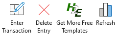
To make the data-entry process simple, there is a userform which will allow you to enter your buy and sell transactions. You can also enter starting balances and dividend payments. You can access the form from the Trading Journal section on the Home tab, right within the Excel ribbon.

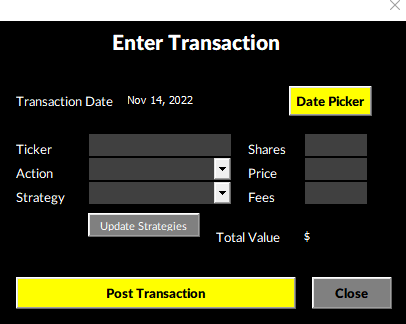
By clicking the Enter Transaction button, you will see the following form pop up:

To start, you can use the Date Picker button to select the transaction date. With the date picker, you can use the button on the left and right side to move one month at a time. You can also select the month from the drop-down list. You can change the year by just typing in the year of the transaction. Once you have the right date and month, use the tab key so that the calendar updates. Then, click on the date the transaction relates to.

Next, select the action type. This will determine which fields you need to enter. There are multiple options to choose from.

- If you are buying a new stock you don’t already own, select Open New Position.
- If you already own a stock and are adding more shares, select Add to Existing Position.
- If you are selling shares of a stock you own, select Sell Shares.
- If you are adding cash to your portfolio, select Enter Contribution.
- If you are withdrawing cash from your portfolio, select Enter Withdrawal.
- If you are recording dividend payments, please select Enter Dividends.
- If you are already own stocks and need to enter in your initial positions, select Starting Balance. For starting cash positions, use the Enter Contribution option.
You will then see a different form based on your selection, showing you which fields you need to enter.
Using different investing strategies
By default, there are three investing strategies you can select from when buying a stock: Buy and Hold, Contrarian, and Speculative. This can be helpful if you want to track how your different strategies work. If you don’t use different strategies, you can just leave everything as Buy and Hold. If, however, you want to add or modify strategies, click on the Update Strategies button when entering a new position:

That will then populate a new userform where you can manage the different strategies.

How the template tracks transactions
When you enter a transaction, it goes into two places. One is the Activity tab, and this acts as a log for everything you’ve entered. There is also the Transactions tab, which is designed for traders to track their opened and closed positions.
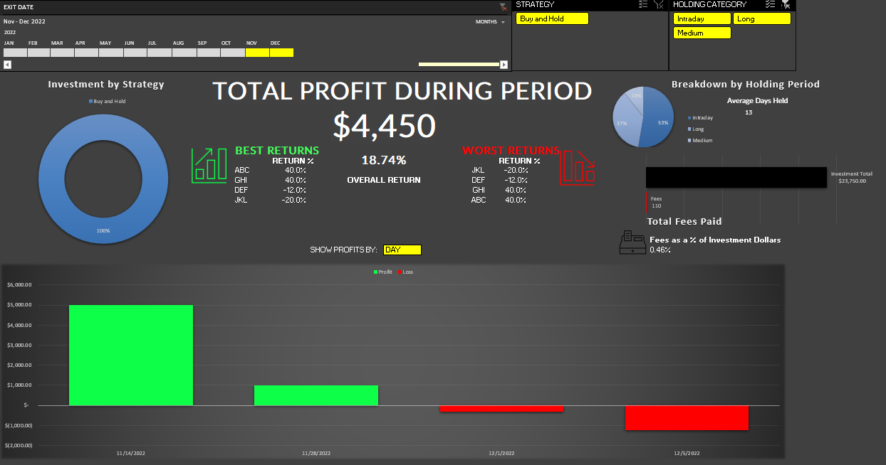
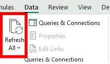
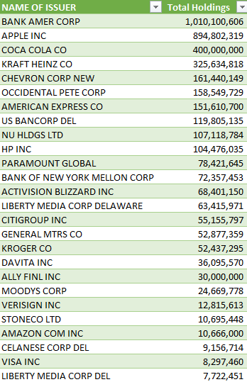
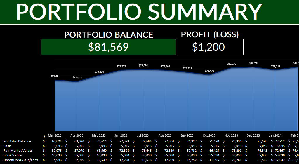
The data also flows through to the Summary tab, where you will be able to see your running portfolio balance, track gains and losses, and also see reports highlighting your overall trading performance. To make sure that all the charts update correctly, click on the Refresh button from the Trading Journal section on the Home tab.
Download the template
Want to try out the template? You can download the trial version here. It is limited to 25 transactions. If you like it, please consider purchasing the full version.
If you run into any issues with the template or have feedback or suggestions for improvements, please feel free to contact me. Please include the name of the template when drafting your message.
If you like the 2024 Stock Trading Template, please give this site a like on Facebook and also be sure to check out some of the many templates that we have available for download. You can also follow us on Twitter and YouTube.