Do you need a calendar in Excel to quickly write down your tasks or keep track of deadlines and appointments? With this free template, you can create a calendar within seconds for the month and year that you want. You can copy multiple tabs and create multiple months in advance. The template will also allow you to specify whether you want the day of the week to start on a Sunday or a Monday. If you would like to try it out, you can download it here.
How the template works
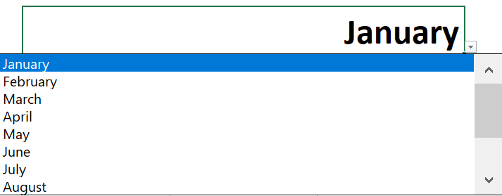
The template only has three areas where you need to make inputs. That includes the month, year, and when you want the week to start. To update the month, simply click on the dropdown in the month field, where you will be able to select from any of the 12 months in the year. You can also type in the month but if you make a typo, then you will get an error.
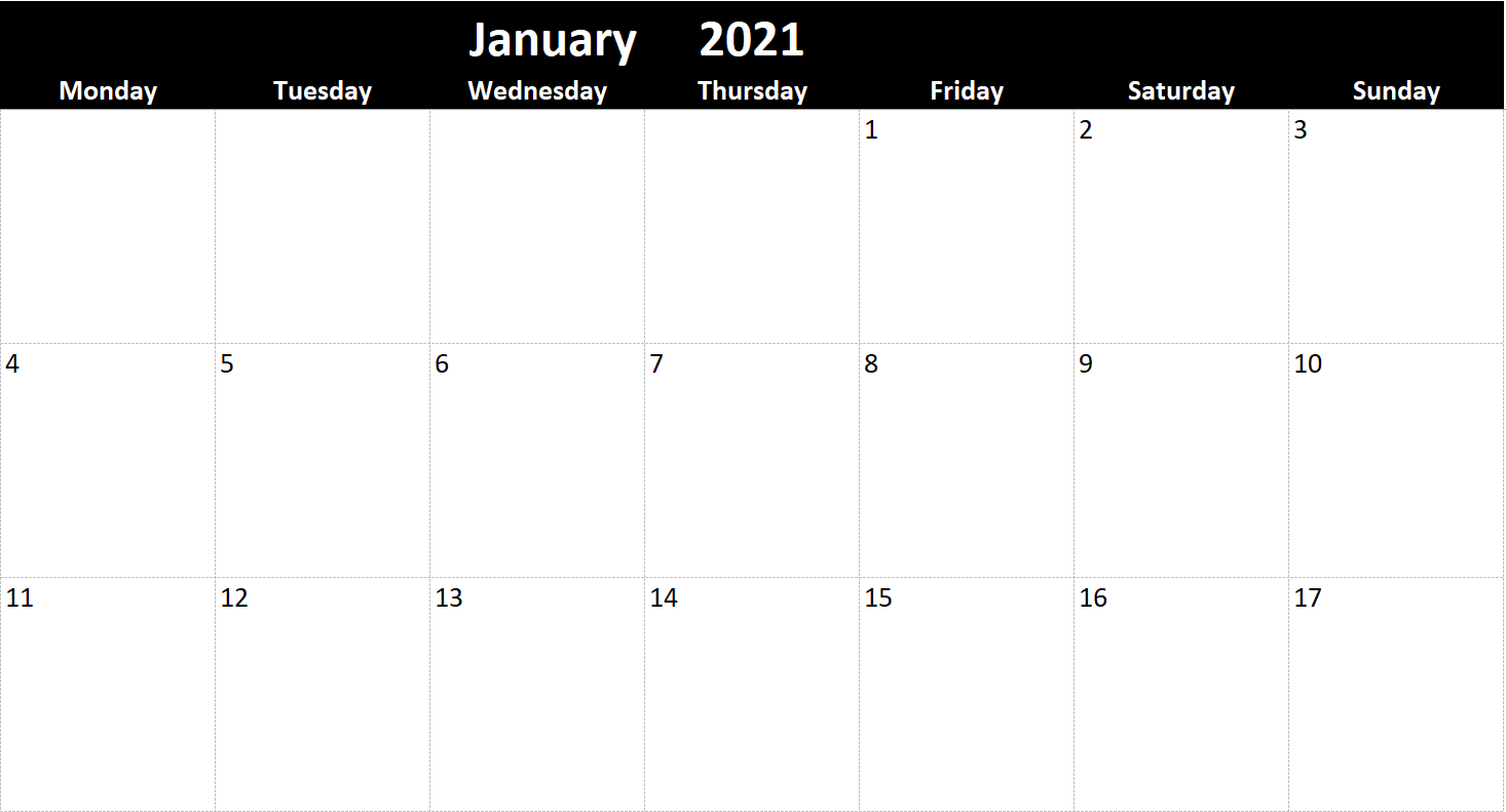
Next up, enter the year for the calendar, which is right next to the month. In this field, you can just enter in a number as a dropdown isn’t necessary here. Then, once you have selected a month and year, the calendar will automatically update based on your selections:
By default, I have the calendar set up to start on a Sunday. But if you prefer for the week to start on a Monday, simply scroll over to the right-hand-side of the sheet where you will see a dropdown. There, you can change the selection and specify which day you want the week to start on:
If I change this to Monday, then my calendar will update again, this time shifting the dates:
If you need to create multiple months, you can simply copy the tab for the calendar over and make the selection for another month and year. Whether you need one, two, or a full 12 months, you can set this up easily with this template. This is a file that you can potentially use forever as you can simply adjust the month and year combinations as many times as you like. There are no limitations as to the number of times you can create, copy, or move tabs.
The template is also set up so that there are five cells for each day, one for each potential task or meeting that you need. If you need to squeeze more into there, what you can do is shrink the font down.
However, the sheet is locked down outside of areas where you can enter in data (including the inputs, and the cells below each day). This is simply to prevent people from accidentally overwriting formulas or otherwise causing the file not to function as intended.
If you liked this post and the free Excel calendar template, please give this site a like on Facebook and also be sure to check out some of the many templates that we have available for download. You can also follow us on Twitter and YouTube.
Whether you’re going on a road trip soon or just want to start planning one, this free road trip planner template can help you with that. Not only can you plot up to 10 destinations, you can factor in breaks, select either a desired start or end time (even if your trip may span more than one day), make notes, and add any points of interest you want to mark along the way. The template will even generate a link for you in case you want to quickly pull up a search of hotels in the area.
If you’d like to give the template a try, download it for free, right here. Below, I’ll go over how it works.
Step 1: Set the initial start or end time
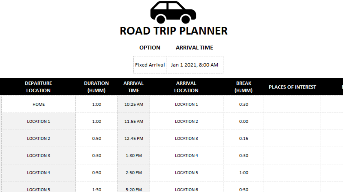
The very first option you’ll find in the road trip planner is whether you want to leave or arrive at a certain date and time. This will determine whether the road trip planner works backwards from your desired ending time or if it starts from your start time and counts forward.
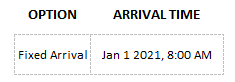
Under the Option dropdown, you can select either Fixed Arrival or Fixed Start. Then, next to that cell, you’ll specify the start or end time, which can include the date — this is useful if your trip is overnight or will be a long one that may include a hotel stay.
Step 2: Enter your arrival locations, duration, break times, and any notes
Now comes the part where you enter the details of your trip. The fields in light grey are formulas and are locked. This is to prevent mistakes and avoid errors. Besides the starting departure location, all subsequent departures will automatically populate based on your last arrival location.
To enter the duration of the trip, make sure you enter it in the following format:
hours:minutes
For example, If a trip will take 30 minutes, you would enter 0:30. If it takes one hour and 20 minutes, the entry needs to be 1:20. This is also how you will enter the break times. The break is simply how long until you plan to resume traveling. And so if you’re staying overnight at a hotel, you might put in eight hours, or 8:00 for a break. The break time will add on top of your arrival time to determine your estimated departure time for your next destination.
If you want to mark places along the way you want to visit in your road trip or just make some notes, you can use these last two columns for this purpose. This might be a good place to mention where you want to fill up for gas.
Additional features
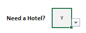
If you want to be able to quickly check the price of hotels in your arrival destinations, click on the the dropdown box after the notes column and select Y for whether you need a hotel:
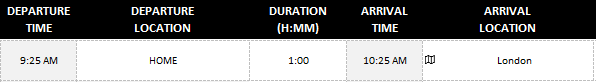
Doing this will generate a link to TripAdvisor’s hotel page for the arrival location that you specified for each line. For example, if my first location was London and I specified Y for Hotel, I would have a link that I could click on to take me to the TripAdvisor page:
It’s a quick way to get to that page and scan hotel availability and rates.
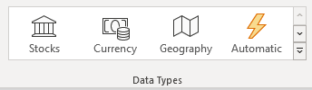
If you’ve got the latest version of Excel, there’s another cool feature you can make use of, and that is its new Data Types (it is location in the Data tab). If I click on the cell for London, under Data Types, I can select the Geography button:
Now, on the cell there’s a little icon indicating a map on it:
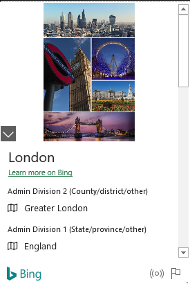
If I click on that icon, I get the following pop-up:
It’s a new feature in Excel that can help you pull up some details on your destination and it gives you a way to bring in even more data into the spreadsheet. However, please note that using this custom data type will break the link for hotels as it will no longer read as a normal text entry.
If you have any suggestions as to other items you’d like to see in this template please let me know. I’m also planning to work on a broader vacation template that considers costs in addition to just travel time.
If you liked this post and my free road trip planner template please give this site a like on Facebook and also be sure to check out some of the many templates that we have available for download. You can also follow us on Twitter and YouTube.
Many people are out buying homes this year as interest rates are at record lows. But figuring out what you can afford can sometimes be a bit challenging. You need to factor in how much of a downpayment you can afford, what your monthly payments will be, and your income. Oftentimes you’ll end up doing multiple what-if scenarios. However, with the free mortgage payment calculator in Excel, you can get a quick snapshot of all the pertinent information to help you determine which house prices are within your range. You can download the template here.
How the calculator works
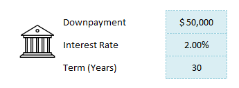
There are three sets of inputs on the calculator. The first section relates to the mortgage itself — how much of a downpayment you can make, the interest rate that’s available to you today, and how many years long your mortgage will be.
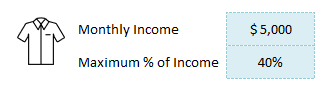
The second section relates to how much income you make as well as how much of your income you want going to cover your mortgage. This is a good way to gauge affordability to ensure that the monthly mortgage payment is within your means. For the monthly income, you’ll want to use after-tax income since this is what will actually be available to you to pay your mortgage payments and other expenses. This is also tied to the worksheet’s conditional formatting. When the % of the monthly mortgage rises above your maximum%, the cells will highlight in red to show that these house prices will be too expensive based on your threshold.
This is an optional section and if you don’t enter it then the spreadsheet simply won’t populate the % of monthly income and there won’t be any conditional formatting applied.
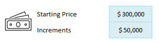
The last section is simply what house price you want to start at, the minimum value that you want to look at. There’s also an area where you can determine at what increments each option should increase by. For instance, if you want to look at a very narrow range, you might put $10,000 to see the different scenarios if the house price increased by $10,000. If you’re looking at a much wider range, you could increment the values by more, such as $50,000 or $100,000.
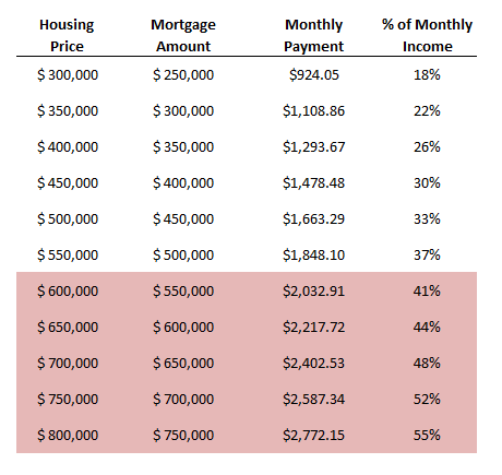
As you enter values in these fields, the mortgage payment calculator will update its results and show you how the different scenarios look like at the different prices.
The above table will be updated immediately as you make changes to your inputs. Please note the spreadsheet is locked and you only can enter data in the inputs. This is to prevent user error and the possibility that formulas are overwritten.
If you liked this post on the mortgage payment calculator in Excel, please give this site a like on Facebook and also be sure to check out some of the many templates that we have available for download. You can also follow us on Twitter and YouTube.
Do you need to calculate the present value of future cash flows or assess two options that will impact your cash flow over many years? Excel’s a great place to do that and below I’ll show you how you can easily set up a template to calculate discounted cash flow that you can adjust for changes in the discount rate and cash flow. And if you don’t want to create your own template, you can download mine at the bottom of this post.
In this example, I’ll compare a lump sum lottery win versus a scenario where you receive an annual amount for 25 years. Step one is knowing to calculate present value, which is what I’ll cover next:
Calculating the preset value
To calculate the present value of future cash flow, you need to know what discount rate to use. What you can use is the rate that you can earn on a typical investment. For instance, if you invest in stocks and assume you can make 5% per year, on average, then you might want to use that as your discount rate. If you want to be more conservative, you could use a rate of 2%. Below, you’ll see how the discount rate can play a big impact in your calculations.
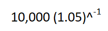
That’s because when calculating today’s present value, you have to use the discount rate to bring the future value back to what it would be worth today. For example, suppose you were to receive a $10,000 payment a year from now, and your discount rate was 5%. An easy way to calculate this is as follows:
You might see other formulas on the web involving fractions to calculate present value but just using a negative power does the trick. This calculation yields a result of $9,523.81. Because you’re not getting the payment today, the value of that money is worth less than the full amount. Consider that if you were to receive $10,000 today and invest it and earn 5%, then a year from now it would be worth $10,500 — more than if you were to receive the $10,000 in a year.
Now, suppose you used a discount rate of just 2%. In that scenario, the $10,000 payment a year from now would be worth $9,803.92 today. Since the discount rate is lower, there’s less of a cost associated with waiting for your payment. If the discount rate was 0%, then there would be no incentive for you to invest your money since a year from now it would still be worth the same value it is today. That’s why when interest rates fall and get closer to zero, people will be less inclined to keep their money at the bank and there’s more demand for gold — since that can be a better way to store wealth at that point.
Creating a template to calculate discounted cash flow in Excel
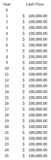
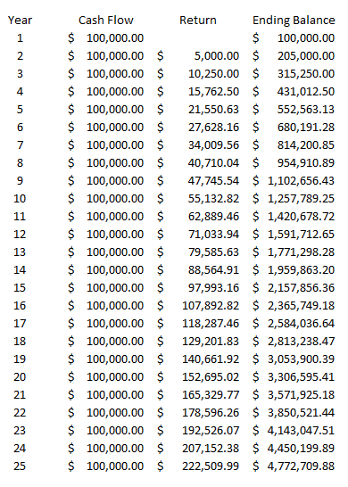
Now that we’ve gone over how to calculate discounted cash flow in Excel, we can set up the template. All that’s really necessary here is to map out the payment schedule, including how much cash you’ll receive every year. Here’s an example scenario of receiving $100,000 for 25 years:
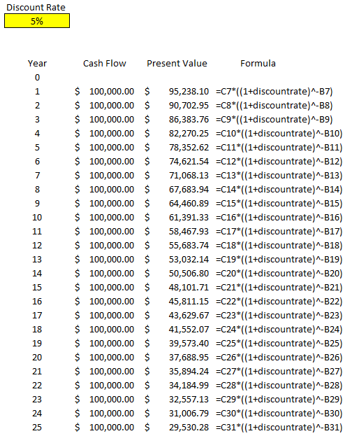
All the payments don’t have to be the same, but for the lottery example, I’m going to keep them that way. What I can do is create another column that will tell me the present value of each one of those payments. To do that, I’ll use a formula that takes the cash flow value, multiples it by the discount rate (I’ll use 5%) raised to a negative power (the year). Here’s how that looks:
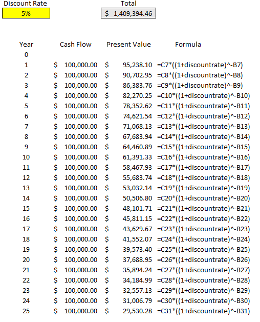
I created a discount rate named range so that it’s easy to reference the percentage and to change it. The only thing left here is to calculate the total of all these payments, to arrive at the present value of all of them:
The total present value of the payments comes in at just over $1.4 million. Even though the total of all the payments over 25 years is $2.5 million, we’re losing a lot of that value because of the time value of money, at a rate of 5% per year.
However, let’s prove this out, and to do that let’s look at the future value of all these payments. Let’s assume that these funds will be reinvested and earning a rate of 5% every year. Here’s how much we’d have by the end of year 25:
In this situation, we’re benefitting from compounding and earning 5% on each year’s ending balance, which includes the prior-year return. By the end of year 25, if we were to invest all of these $100,000 payments at a rate of 5%, we’d have a future ending value of $4,772,709.88.
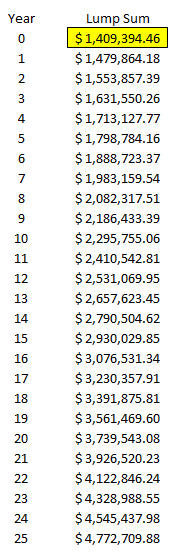
Now, remember, the equivalent of these annual payments is a present value of $1,409,394.46. Let’s assume that rather than receiving annual payments of $100,000, we simply receive a lump sum payment of this and invest it and also earn 5% every year. Here’s how that will look like:
The ending value after 25 years is the same, $4,772,709.88. This tells us that if you’re given the option of 25 annual payments of $100,000 or a lump sum of $1,409,394.46 today, there’s no difference to you (if the discount rate you’re using is 5%). If the discount rate is 2%, then the present value climbs to $1,952,345.65.
As you can see, depending on which discount rate you use, it can have a significant impact on your present value calculations. This template will allow you to quickly change the discount rate and see how the calculation looks under different scenarios. You can also add more years to this calculation by just extending the formulas down. The amounts also don’t need to be identical, they were only set up this way purely for the purpose of comparing lottery winnings in a scenario where you earn one lump sum amount versus equal payments over multiple decades.
If you’d like to download this template to follow along, the free version is available here, which goes up to year 15. For the full and unlocked version, which has no ads and goes up to 30 years, please refer to the product page here.
If you liked this post on how to calculate discounted cash flow in Excel, please give this site a like on Facebook and also be sure to check out some of the many templates that we have available for download. You can also follow us on Twitter and YouTube.
Several weeks ago, I discovered that Excel had a new function called STOCKHISTORY. It’s able to pull stock prices and a great way to track stock prices and can help calculate returns. Excel does make it clear that it is not for trading purposes. However, it’s still a great way to stay on top of tracks and see how they’re performing. Below, I’ve created a template that will allow you to track stock prices and arrange them from best-to-worst.
Note that for this template to work, you need to have the STOCKHISTORY function on your computer, otherwise you’ll get nothing but errors. So your first step will be to check if it works on your file. Refer to the original post on the function as it will also explain how you can get it on your computer if you don’t already have it. If you’re running on old versions of Excel, you’re out of luck.
But for those that aren’t and that have access to the function, read on.
Entering the ranges that you want the macro to sort.
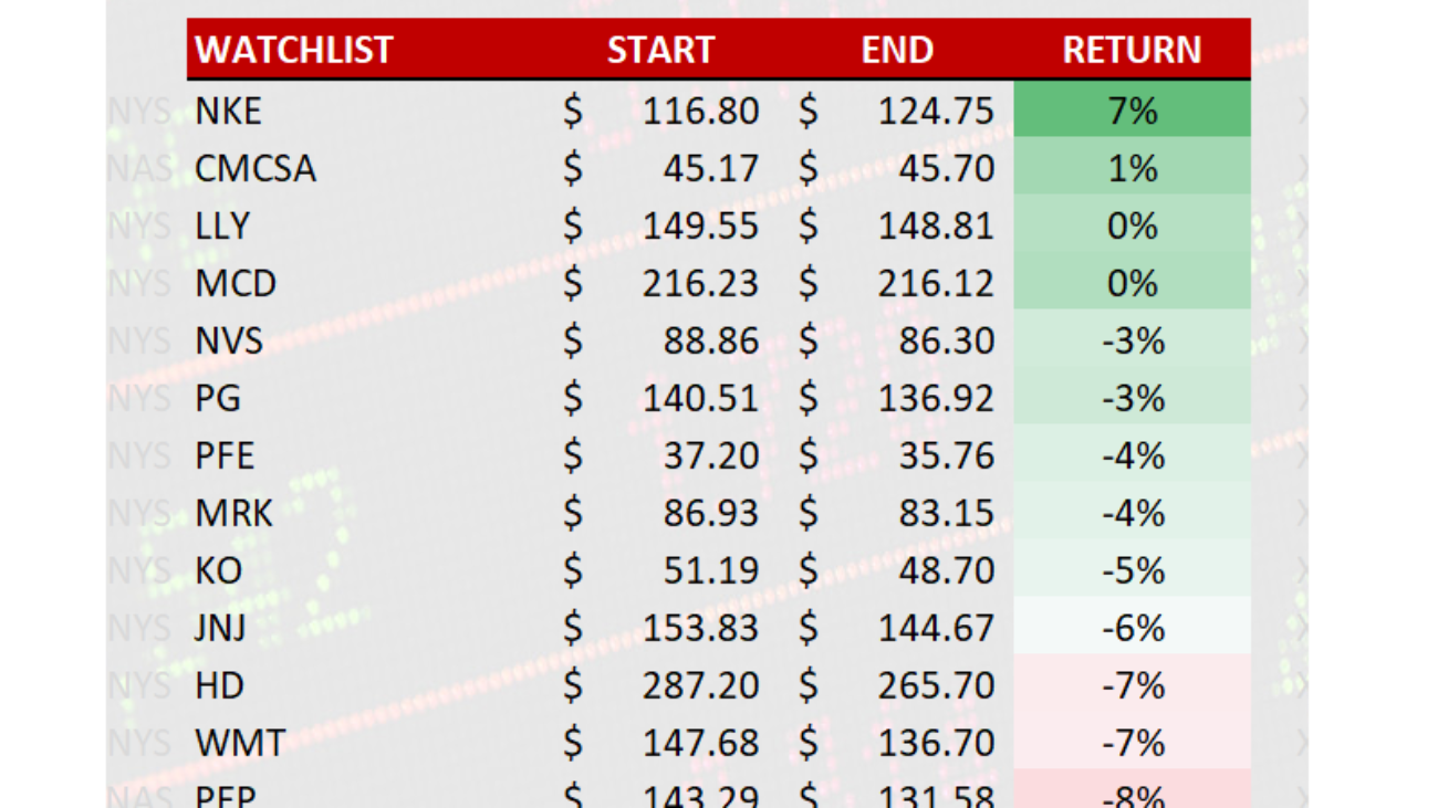
Let’s start with the first one, selecting stocks. I’ve already created three stock sections in this template, which you can of course change. Let’s look at one of them as an example:
The Start, End, and Return values are formulas. The only things you need to enter are the ticker symbols. Off to the left, shaded in light grey, I’ve also entered the code for the exchange. For the New York Stock Exchange, it’s XNYS, while the NASDAQ is XNAS. For a full list of the codes, refer to the original post on the STOCKHISTORY function. If it’s a popular stock that’s on one of the major exchanges, you may not need to enter it. I’ve included the exchange code for the sake of avoiding errors as it’s possible Excel might not know which ticker you’re looking for and select the wrong one.
You can extend the ranges to accommodate more tickers, you’ll just need to copy the formulas down in the Start, End, and Return sections.
Next: the date ranges.
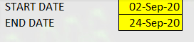
Off to the right of the template, there’s a section where you can enter the start and end dates.
The template will adjust for weekends but not for holidays. If you see a #VALUE! error in the values, that likely means there’s an issue with the date, so you’ll just need to change one of the dates to ensure it doesn’t fall on a holiday.
Lastly: the ranges to sort.
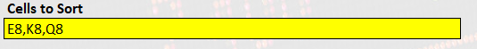
To the right of the dates, there’s another area where you can enter which cells to sort:
Cells E8, K8, and Q8 on this template are where my ‘RETURN’ headers are located, and where the percentages are. If you add sections or modify this template, you’ll need to update the cells to sort. When you update the start or end dates, the template won’t automatically re-sort until you click on this button:
If you get an error on the re-sort button, make sure you check which cells are in the Cells to Sort area and ensure that they’re correct.
#CONNECT! errors
One thing you may run into on this template are #CONNECT errors. I’ve noticed this happens once you start adding too many ticker symbols. Sometimes it’s hit or miss and you’ll get all the prices updated, but if you’re planning to list every ticker out there, just be forewarned that you might run into issues here. It’s a separate error from the #VALUE! error and one that can’t be fixed through the template, without removing some ticker symbols, anyway.
If you liked this post on the StockHistory Template, please give this site a like on Facebook and also be sure to check out some of the many templates that we have available for download. You can also follow us on Twitter and YouTube.
If you’re an accountant, you know that quickly doing a t-account can sometimes help you plan your journal entries and save you some headaches later on. But sometimes it can be time-consuming and a bit cumbersome to go through the process of setting everything up in an Excel spreadsheet. That’s where my new, live t-account template can help you.
Simply go to this link and you’ll be taken to a page where you can start creating your t-accounts on the fly. All you need to do is first make sure you name the accounts along the top and then record the entries on the left-hand-side. The accounts will automatically update as you enter the data.
Here’s a quick demo of how the page works:
It supports 20 line items and five accounts. And if you make a mistake or want to make another set of t-accounts, you can just refresh the page to clear what you’ve entered.
If you like the live t-account template and find it useful, please give this site a like on Facebook and also be sure to check out some of the many templates that we have available for download.
Unless you’re still stuck on old versions of Excel, you probably know that you can filter data using colors. And by doing so you can use the SUBTOTAL function in excel to tabulate those amounts. But in this post, I’m going to show you something a little different. By using a macro, I’ll highlight cells containing values and then sum them by color in Excel, without needing a subtotal or a filter. This free template will just use VBA to populate the totals.
How the template works
In this template, all you need to do is enter your data and then assign whatever formatting you want to use to identify a cell to the corresponding category. As long as a cell has the exact same formatting as the category, it will be included in that category’s calculation.
I got the idea when I was trying to quickly analyze expenses and didn’t want to go through a whole process of putting it into a complex budget template. Rather than setting up logic to classify whether an expense falls into one category or another, I thought color-coding could be another way you could quickly group expenses.
Here’s a quick video showing you the template in action from color-coding cells to calculating the totals:
Setting up the data
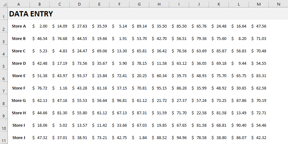
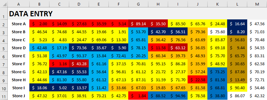
In the template, there’s one section dedicated to the raw data where you’ll enter your inputs:
You can input data up until column N, although I’ve left the column blank for a buffer. In this example, I’ve put in random numbers and grouped them based on a store value in column A. This can be all numbers, it doesn’t really matter, I just preferred to have some grouping.
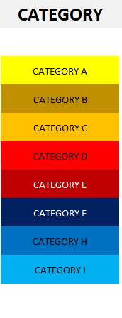
Next to the data entry, I’ve got a list of categories set up in column O:
You can add as many categories as you like. How they’re color-coded here is how you’ll need your cells will need to look to ensure they’re in the correct categories. For instance, any cells that are highlighted in light blue will go into Category I. Whereas anything in a dark red will belong to Category E.
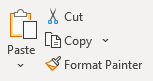
You may think this would be a painful process to try and color-code your data based on all these different categories. After all, what if you get the shade wrong or the font color is wrong. The solution’s really simple and you just need to use our trusty friend, the Format Painter. If you’re not familiar with it, this is what it looks like:
It’s on the left-hand-side of the Home tab where the copy buttons are. What you can do is select the category you want to be assigning data to, click once on the Format Painter and then click on the cell you want to highlight with that exact same formatting.
If you’ve got multiple cells that you want to apply the formatting to and don’t want to keep repeating this exercise, then Double-Click on the Format Painter. You can now continue selecting cells and the Format Painter will take care of the formatting for you. You won’t need to re-select it each time. Once you’re done with the formatting and want to stop applying it, click on the Format Painter again to stop.
I’ve color-coded some of my data based on the categories, and here’s how it looks:
Updating the calculations
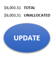
On the right-hand-side of the page there’s a button that says Update. This will update the totals based on the color-coding. You’ll need to have macros enabled for this to work. Above the button you’ll see the total of all the values in columns and how much is unallocated.
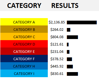
Clicking on the update button will trigger the macro to run the calculations. After pressing the button, here’s what my categories look like and the totals corresponding to their color-coding:
You’ll notice I’ve also created visuals to see the relative size of each category using the REPT function. If you’re interested in learning how to use this function, check out this post.
Anytime you make changes to the color-coding, be sure to hit the Update button. I didn’t want the formulas to update every time there was a change on the sheet because that can sometimes slow a spreadsheet down, especially since it would involve recalculating all the totals.
The code
Here’s the VBA code itself on how the update button works:
Sub Oval1_Click()

Dim clvalue, clcolor As Double
Dim cl, colorrange As Range
Dim lstrow As Integer

lstrow = ActiveCell.SpecialCells(xlLastCell).Row

Set colorrange = Range("colorrange")

'clear data range
colorrange.Offset(0, 1).ClearContents


For Each cl In ActiveSheet.Range("A1:O" & lstrow)

    If IsNumeric(cl) Then

        clcolor = cl.Interior.Color

            For Each lookupcl In colorrange

                If lookupcl.Interior.Color = clcolor Then
                    lookupcl.Offset(0, 1) = lookupcl.Offset(0, 1) + cl.Value
                    GoTo nextcl:
                End If

            Next lookupcl
    End If

nextcl:

Next cl

End Sub
There’s a named range called “colorrange” that it cycles through, and those are the categories in column O on the spreadsheet.
Using the template
This isn’t a terribly complex template to use. However, it can help if you want to quickly group items. It’s a unique way to classify expenses rather than just using drop-downs and complicated formulas. And it makes it easy to sum data by color in excel. The way I found it useful was to list your vendors or stores in column A. Then, arrange transactions by date (e.g. the first transaction is in column B, then C, and so on). But this can be used in a variety of different purposes to help classify data.
If you want to reset the calculations, just change the data back to the default formatting or something that doesn’t correspond to a category you already have, and then click update.
Download
The template is free to download and it’s available here.
If you liked this post on how to sum by color in Excel, please give this site a like on Facebook and also be sure to check out some of the many templates that we have available for download. You can also follow us on Twitter and YouTube.
If you earn income from multiple jobs, you know how important it is to keep track of how much you’re making. If you work too little, you may not be making as much as you were planning. And if you’re working a lot more, you could afford to give yourself a break.
Whether you’re self-employed or you supplement your income by driving for Skip the Dishes or Uber, there’s no shortage of ways to make money these days which doesn’t involve working a regular 9-to-5 job. The income tracking template I’ve created will allow you easily track your income from various sources and help you stay on track if you’re targeting a certain income figure for the month or year.
There are two tabs on this template: inputs, and calendar. The inputs are where you’ll go to enter in your income, so let’s start there.
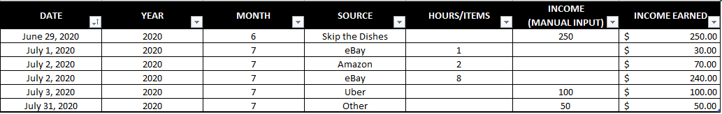
On the Inputs tab you’ll enter the date you earned the income, the source, and how much you made. You can setup hourly or item rates. You can also just enter in a fixed income amount. Here’s an example of some sample inputs:
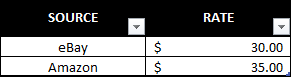
For jobs like Skip the Dishes or Uber where you don’t earn an hourly wage, you’ll need to enter a manual amount. If you sell items on eBay or Amazon where you might have an average price, you could potentially use a rate. And that’s where the rate schedule comes in handy:
This could also work if you work a part-time job or something where the rate is fairly steady. Whether it’s per hour or per item is irrelevant. The point is to try and make the input section as easy as possible and you don’t need to necessarily use the rate schedule if you don’t need it.
But if you enter a number under the hours/items section, the income earned formula will be looking for a rate to multiply that by — you’ll get an error if it can’t find one (unless you enter a manual total, which will override the calculation). So if you don’t have a rate for that source of income, don’t enter anything in the hours/items section and just use the manual input column.
Once all your data’s entered in, it’s time to head over to the Calendar tab.
A summary of all your income
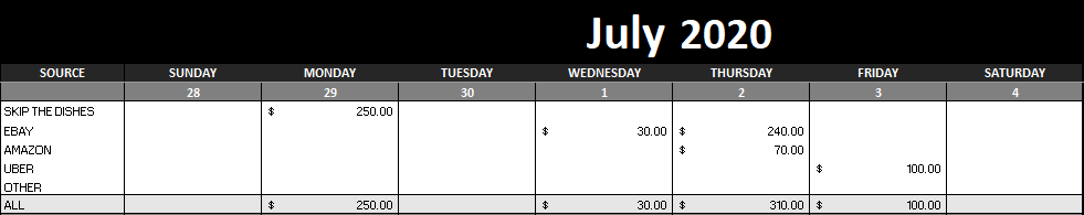
For the week that I entered the weekly income for, here’s what the calendar shows:
You can visually see how much you’ve made each day and there is also a weekly total at the end. The key to everything calculating correctly is the value in the source column needs to match what you entered on the inputs tab.
There’s also a column further down titled Annual Run Rate which will tell you how much you’ll earn over the course of the year if you work a full year at your current weekly pace.
It’s simply a way to gauge whether you’re on track that week for your annual goal or not. That brings me to the next section: the setup.
Settings and goals for the income tracker template
If you scroll over to the right on the calendar tab, you’ll see an area where you can specify a number of different settings and goals. Only change the items that are highlighted in grey. Let’s go over each one:
Work weeks. This is how many weeks you plan to work during the year. If you are going to work every week then you can leave this at the default value of 52. If you’re going to take some weeks off, then deduct from that total. The purpose of this is for calculating the annual run rate.
Include partial month. If you strictly only want to include the days that fall in the month when calculating your weekly totals, then set this to ‘N’. If you set this to ‘Y’, then the first and last weeks of the month could include parts of the previous and upcoming months, depending on where the month ends and starts. The purpose of setting it to ‘Y’ would be so that every week is a full week. For instance, July 2020 began on a Wednesday. If you set partial months to ‘Y’, then your July calendar and weekly totals would include June 28-30. If you set partial months to ‘N’, then those days would not show up on the calendar and they wouldn’t be included in your weekly totals.
Monthly goal. This is the total income you want to earn on a monthly basis.
Annual goal. This is the total income you want to earn for the full year.
Below the setup options, you’ll also see a summary of your sales by month. You can enter the year if you’ve got multiple entered. But by default, I’ve set this to 2020.
Tracking your goals
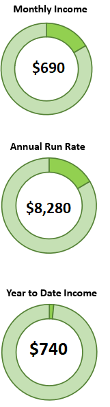
Next to the calendar, you’ll also see charts showing you the progress that you’re making relative to your goals for the month and year:
The different gauges show different things. The first one is how close you are to reaching your monthly goal. The next one is how close you are to your annual run rate based on the monthly income you’ve earned thus far. And the third takes a tally of all of the income you’ve entered on the inputs page and compares it to your annual goal.
Download the template
This template is free to use and allows you to stay on top of all your income sources. The version is locked down to minimize data entry errors and does come with an ad. But as it is, it will allow you to enter in your data and the template is fully functional. You can download it here.
Currently, the template supports five income sources and you can adjust those in the free version. With the premium version, everything is unlocked and there is no ad. And you could add more income sources on the calendar tab if you’re comfortable adding rows and updating the formulas.
If you liked this post on the income tracker template, please give this site a like on Facebook and also be sure to check out some of the many templates that we have available for download. You can also follow us on Twitter and YouTube.
A countdown timer can help you track how much time there’s left to do a task or until a deadline comes due. Below, I’ll show you how you can make a countdown timer in Excel that can track days, hours, minutes, and seconds. In order to make it work, we’ll need to use some VBA code, but it won’t be much. And if all else fails, you can just download my free template at the end of the post and repurpose it for your needs.
Let’s get right into it and start with the first step:
Calculating the difference in days,
To calculate the difference between two dates is easy, as all you’re doing is subtracting the current date and time from when you’re counting down to.
The start date is just going to be today, right this very second. And Excel has a convenient function just for that, called NOW. It doesn’t require any arguments and all you need to do is enter the following formula:
=NOW()
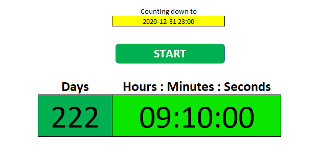
Entering the date and time you’re counting down to is a bit trickier. As long as you enter it correctly, then calculating the differences will be a breeze. However, this may involve a little bit of trial and error since it’ll depend on how your regional settings are setup. For the countdown date, I’m going to set it to the end of the year. Let’s say 11:00 PM on New Year’s Eve. Here’s how I input that into my spreadsheet:
2020-12-11 11:00 PM
The key things to remember here are that there should be a space between the time and the AM/PM indicator (if you use it) and there should be two spaces between the date and the time. Then, it’s just a matter of whether you’ve got the right order of date, month, and year. This is where you may need to do some testing on your end to ensure you’ve got the correct order.
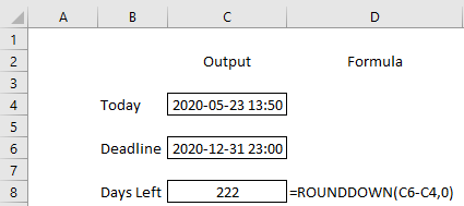
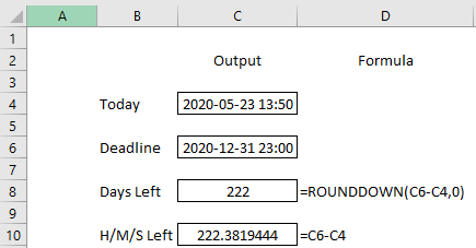
Now that the dates are set up, we can calculate the difference in days. To do this, we can just calculate the difference and use the ROUNDDOWN function to ensure we aren’t adding partial days:
There are 222 days left until the end of the year. By using the NOW function, the formula will automatically update and tomorrow the days remaining will change to 221, and so on. If your output’s looking a little different, make sure to check the formatting and that it’s set to days.
Calculating the difference in hours, minutes, and seconds
There’s not a whole lot of complexity when it comes to calculating the difference in hours, minutes, or seconds. We’re still subtracting the current date from the deadline. The only difference is that now we’re just going to change the formatting. If I do a simple subtraction, I end up with a fraction, which isn’t really usable in its current format:
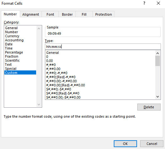
The trick here is to change the format of this cell so that it shows me hours, minutes, and seconds. And that’s an easy fix. If I just click on cell C10 and click CTRL+1, this will get me to the Format Cells menu. In here, I’ll want to select a Custom format so that the cells just shows hours, minutes ,and seconds:
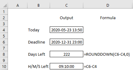
Here’s what the countdown timer looks like after the format changes:
It’s important to include a date in the calculation even though we’re just doing a difference between hours, minutes, and seconds. Otherwise, the formula wouldn’t correctly calculate in all situations, such as when the deadline hour is earlier than our current hour.
Putting it all together
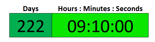
Now that all the calculations are entered in, now it’s just a matter of formatting the data. We can create a countdown clock that separates days remaining, from hours, minutes, and seconds remaining.
One cell can have the difference in days, while another will have the difference in hours, minutes, and seconds. This goes back to just modifying the formatting and applying a custom format. Here’s how mine looks:
Although we’ve gotten to this point, the challenge is that this countdown timer still doesn’t update on its own. Unless you want to click on the delete button all the time, the countdown isn’t going to move unless there’s something to trigger a calculation in Excel. That’s why we’re going to need to add a macro to help us do that, which bring us to the important last step of this process:
Adding a macro to refresh every second
We need a macro to update the file. Whether it’s every second, every five seconds, it’s up to you. While the countdown timer will update when someone enters data or does something in Excel, that’s not much of a countdown. This is where VBA can help us. If you’re not familiar with VBA, don’t worry, you can just follow the steps below and copy the code.
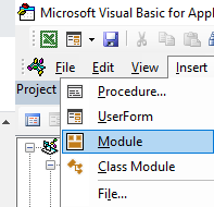
To get into VBA, click on ALT+F11. From the menu. Once you’re there, click on the Insert button on the menu and select Module:
Over to the right, you’ll see some blank space where you can enter in some code. Copy and paste the following there:
Sub RunTimer()

    If Range("C10") <> 0 Then
        Interval = Now + TimeValue("00:00:01")
        Application.Calculate
        Application.OnTime Interval, "RunTimer"

    End If
End Sub
One thing you may to change is the reference I made to cell C10. Change that to where you have your countdown timer. As long as there’s a value in the cell, the macro will continue running. All it does is check if there’s a value there, and if there is, it updates the worksheet every second. And by doing that calculation, your countdown timer will update even if you’re not making any changes to the spreadsheet.
You can also change the interval which currently updates every second, as noted by the 00:00:01. You can change this to five seconds, 10 seconds, however often you want it to update.
But there still needs to be something that triggers the macro to start running. You can assign a button or shortcut key to do that.
However, in this example I’ll activate it when the sheet is selected. Inside VBA, you should see a list of worksheets. Double-click on the one that contains your countdown timer:
You’ll again see blank space to the right where you can enter code. And you’ll also see a couple of drop-downs near the top that you’ll want to look for. By default, the first one should say (General). Change this to Worksheet:
Next, change the other drop-down which will probably say SelectionChange. Change it to Activate. Then you should see something like this:
Copy the following code into there to call the macro we created above:
RunTimer
Now when you switch to another worksheet and come back to the current one you’ll notice your countdown timer is updating on its own. If you want it to stop it, just clear the cell that has the timer. Otherwise, the macro will continue running every second.
The Countdown Timer Template
If you’d rather just use a template, then you can download one that I’ve made here. You don’t have to worry about macros and instead you just need to enter the end time; the time that you’re counting down towards.
I’ve also got a start/stop button that you can toggle to get the countdown timer going and that will pause it:
You can move the button as well as the time your counting down to onto another sheet if you don’t want someone altering it. If you have any questions or comments about this template, please send me an email at [email protected]
If you liked this post on how to make a countdown timer in Excel, please give this site a like on Facebook and also be sure to check out some of the many templates that we have available for download. You can also follow us on Twitter and YouTube.
A word search can be a great way to pass the time and for kids, it can help them practice their spelling as well. With this free word search maker, you can easily create a random new word search in just seconds. With small, medium, and large sizes to accommodate different ages and skillsets, the template provides a lot of flexibility. You can download it here.
Let’s jump right into it and see how the template works:
How to create a word search using the template
There are three tabs in this template: WORDSEARCH, WORDSEARCH.MED, and WORDSEARCH.SM. They indicate their size and difficulty. If you want to create something fairly simple, then the small (SM) tab will work best and it can accommodate up to 10 words. The medium (MED) tab is a bit bigger and you can have up to 15 words. And the main tab will allow you to plot up to 20 words.
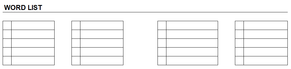
Below the actual word search, you’ll have a list of spaces where you can enter your words in, titled Word List:
Each list contains a pair of boxes. The small one off to the left is where you might tick off that a word has been found. The larger box on the right is where you will enter the actual word.
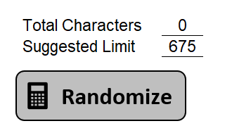
Further off to the right, you’ll see how many characters your words have taken up as well as a suggested limit:
If you’re over the suggested character limit then the macro may have trouble finding space for all your words. If that happens, you’ll get an error message saying so. However, you can still try and see if it’ll work. to create a new word search, click on the Randomize button shown above. This will plot your words randomly in every possible direction, up, right, left, down, and diagonally as well.
Once the words are plotted, then the remaining spaces will be filled in with random letters. However, not every space will be a random mix of any possible letter in the alphabet. Less common letters like Z, X, and Q won’t have the same odds of showing up as more common letters. This is done in order to make the word search more challenging.
When the word search is entirely populated you can just print it off. You won’t see where the words were plotted on the word search without actually searching for them yourself. So if you wanted to create a word search for yourself, that’s entirely possible as even the person who runs the macro won’t have any advantage of knowing where the words were placed.
If you liked this free word search maker template in excel, please give this site a like on Facebook and also be sure to check out some of the many templates that we have available for download. You can also follow us on Twitter and YouTube.