admin, Author at HowtoExcel.net

How to Setup Conditional Formatting (including Formulas)

June 7, 2017

by admin with 5 Comments conditional formatting formatting intermediate

Conditional formatting is useful for highlighting cells or ranges if a condition is true. For example: highlighting negative values as red or positive ones as green. You can also do more complex formatting like highlighting an entire row if it meets a criteria.

Creating A New Rule

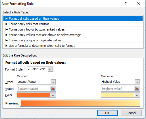
To get started with conditional formatting, you need to select new rule from the conditional formatting options which is under the Home tab:

You will then have quite a few options as to what you want to do:

conditional formatting all cells based on values

Format All Cells Based On Their Values

This is useful if you want to show some sort of progression from one value to the next, as one colour will fade into the next. Here is an example using this conditional formatting on a range of values from 1 to 5:

1 started from the dark orange and gradually got to a light yellow colour by the time it got to the number 5. You can change the colours involved or even the range. You also can change the values instead of using lowest to highest values you can hardcode figures, use percentages, or whatever else. In all likelihood it will show something very similar regardless what you select, so leaving it to the default setting here (low to max) is going to be sufficient in most situations.

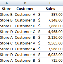
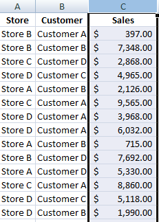
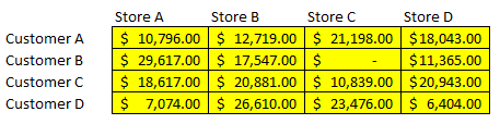
Another way you could use this formatting is if you wanted to compare a time-series. Assume the below are sales numbers and you wanted to highlight good and bad years.

You can see in this example there is no longer the smooth transition as in the prior example since I’ve assumed sales are bouncing up and down. The downside of using this type of conditional formatting as you could have a really colourful dataset if you did this.

You may like it initially but if you are dealing with lots of data it may not be all that helpful because you are dealing with many different shades of colours now and you may find yourself comparing different shades to see if one is darker than the next. And conditional formatting is most useful when you don’t have to spend time analyzing colours, and instead the colours help you do the analysis by easily standing out and highlighting what you want to see.

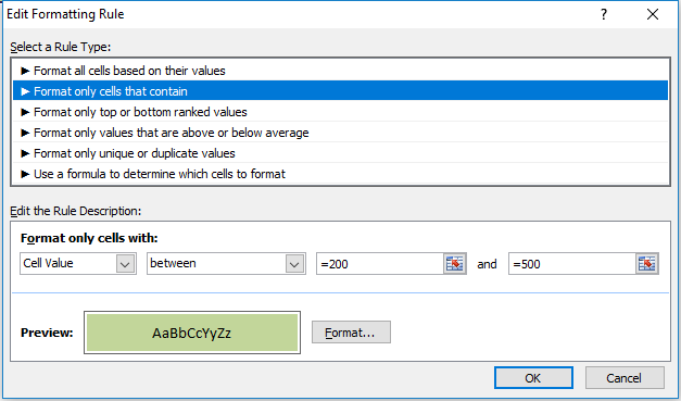
Format Only Cells That Contain

The next option on the formatting rules allows you to specifically look at the cell values. Keeping my sales numbers example from above I want to highlight cell values from 200 to 500. In this case I only need to select between and a low value of 200, and a high of 500.

Now unlike the format all cells example, the remaining conditional formatting rules require you to explicitly set what formatting you want to apply, it won’t just smooth colours from one to the other. And every cell in the range won’t have conditional formatting on it unless I explicitly state it. To set the formatting for I want cells that fall in this range to be I just click on the Format button below and apply what formatting I want. In this example I just set the cells to be highlighted in green.

(Note you do not need to put the = sign before the number, it automatically does this after you have already setup the conditional formatting.)

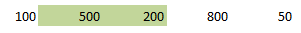
Below is my result

The cells that do not fall within this range do not have highlighting. If I wanted them to have highlighting I would have to change the rule, or add another rule for them. So what I will do is add another rule for any values under 200:

In this case I set the formatting to be light red.

Please note you still want to make sure your range is selected when you are adding a new rule so that it gets correctly applied to the range. Otherwise you will need to adjust the conditional formatting settings so that they are applied to the correct range.

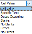
Both the drop downs that currently contain Cell Value and less then can be changed. Cell Value can be changed to the following:

If you change this value then some of the options for the next drop down will change as well. Obviously you cannot choose less then or greater than operators when dealing with text. There are a lot of possibilities here so you can experiment with them by changing these drop down selections. Currently, for the Cell Value selection, these are the different operators available:

Going back to my example here, I selected the less than operator since I wanted to highlight values that were under 200. My result is the following output:

conditional formatting between less than

Now I have formatting for every number except 800. So I could make a similar rule and set that one to anything over 500.

The disadvantage of using the formatting based on values in the first example is that not all your values have conditional formatting on them. But this could be an advantage as well as it allows you to have more control over the exact type of formatting you want. Here I can have green and red which helps to quickly distinguish the results without having to closely look at the shading.

Format Only Top Or Bottom Ranked Values

This formatting option allows you to just highlight your top or bottom values.

conditional formatting top ranked values

I have selected the top 10 to be highlighted in green and as a result I get the following:

The problem here is I don’t have more than 10 values so everything will be highlighted. In fact, even if I were to select bottom 10 then that would apply to everything as well.

One way around this is to check the box for % of the selected range. now it will look at the top 10% rather than just the top 10 values.

Now my highlighting looks as follows:

What this effectively does now is look at the percentiles and pulls the top 10%. So if I had a data set of 20 values, it would highlight the highest two values.

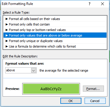
Format Only Values That Are Above Or Below Average

This option will just compare the value against the average.

conditional formatting above below average

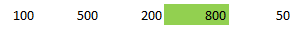
If I select that it highlights anything above the average I will get the following result:

The average for this data set is 330, so it correctly has highlighted the values 500 and 800.

Format Only Unique Or Duplicate Values

This is probably the simplest formatting option where you have only one of two options – unique or duplicate.

In my example all of my values would be highlighted since none are duplicates.

Use A Formula To Determine Which Cells To Format

This is the most versatile option for formatting. But also is the one that will take the most time to setup. In an earlier post I showed how to use this option to create highlighting on alternate rows.

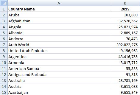
In this example I’ve downloaded Alphabet’s financials from Google Finance for the past five quarters. This is what it currently looks like:

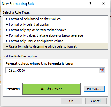
I will start with setting up a rule to highlight every column where income after tax is more than 5,000. To do, I will select cell B11 and setup the following rule:

I have frozen row 11 since that is where the after tax numbers are, and I want these figures to change based on what column I am in, but not what row I am in. So for that reason I am freezing the row and not the column.

I selected cell B11 when entering this formula because I wanted to be in the same column because when I go to re-size the cells that I want this formatting to apply it to, it will adjust the formula. So if I was in column C and entered my formula as above (referencing column B) then if I change the range I want to apply it to, say columns B:F rather than just the cell I was in in column C, the cell it will be evaluating now will be A11, rather than B11. It will reflect the fact that my range has changed (unless of course I wanted to freeze the column as well but that would not be helpful in this situation).

Which brings me to the next step: applying this to the relevant columns. Initially when you setup rules for conditional formatting it by default assumes you are applying them to the range you have selected. So I could have selected the range B:F but I can just go back into my conditional formatting rules and change the range:

Now this rule will apply to all the columns from B to F. As a result, my updated data set looks as follows:

Now every column where Income After Tax was more than 5,000 has been highlighted.

The easiest way to understand formulas in conditional formatting is this: treat it as an IF function, except start from the logical test argument and ignore the values that they will be if they are true or not. After all, if it is true, the formatting applies, if it is false, it will not apply. In the above example my IF function would have been something along the lines of this:

=IF(B$11>5000,X,Y)

Where X is the conditioning applies, and Y is that it doesn’t.

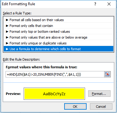
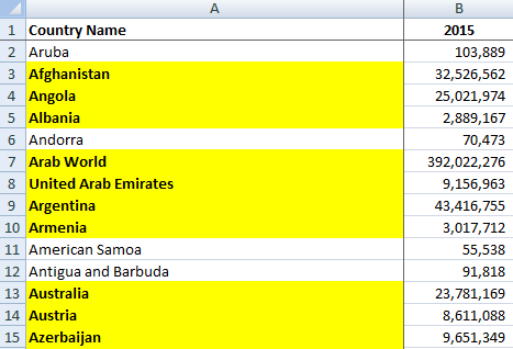
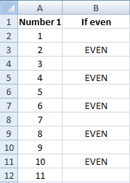
I will apply this logic to use a length (LEN) function. For no logical reason whatsoever, I am going to highlight all the rows that have descriptions in column A that are both longer than 20 characters and have a comma in them. If I were going to use an IF function, the formula would look as follows (in cell B1):

=IF(AND(LEN($A1)>20,ISNUMBER(FIND(“,”,$A1,1))),X,Y)

If I were to apply it to conditional formatting it will look as follows:

As you can see it’s a copy and paste from my IF function, just the logical test argument. I enter this in cell B1 just to make sure the referencing doesn’t change and then I apply it to columns B:F and my data set now looks as follows:

Managing Multiple Formatting Rules

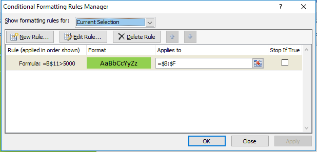
I have an overlap now in rows 3 and 5 as they are highlighting the areas that were previously highlighted in green. If I wanted to change this to make those back to highlight in green I can change the hierarchy of my formatting rules. I can change this by going into Conditional Formatting -> Manage Rules.

If you do not see any rules even though you have set them up, make sure at the top where it says Show formatting rules for that This Worksheet is selected. See below:

If the range selected above is not correct then you may not see your conditional formatting rules.

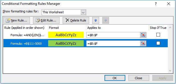
My rules look as follows:

I can change the hierarchy by selecting the green highlighting criteria and clicking on the up arrow to move it above the yellow highlighting criteria. That will mean the green highlighting rules will be applied first. That still won’t keep it green since it just means the yellow highlighting criteria will be applied afterward. This is also the screen where you can delete any formatting you no longer want.

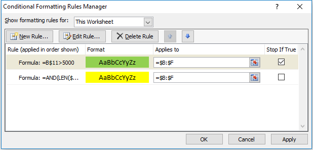
Instead, what needs to happen is for the Stop If True field to be ticked off for the green highlighting rules:

conditional formatting rules manager stop if true

Now the green highlighting is first and if the condition is met the yellow highlighting rules will not run. Now my data set looks as follows:

The yellow highlighting rules have now only been applied to the columns where the green highlighting did was not. By using the Stop If True and setting your hierarchy for formatting you can prioritize what formatting you want to be applied.

Mortgage Calculator – Calculate House Price, Monthly Payment, and Gain or Loss

May 31, 2017

by admin with No Comment template

Download template

This mortgage calculator will allow you to accomplish three different things:

1) Determine the housing price based on a desired monthly payment, interest rate, and terms.
2) Determine the monthly payment based on the price of a house, interest rate, terms, and down payment
3) Calculate the mortgage balance remaining and calculate a gain or loss depending on the selling price you enter.

To select which calculation you are after selecting the option from the drop-down under the ‘Calculate’ header:

All of the inputs are in yellow cells and can all be changed. Please note that since some of the same fields are used in the different calculators, if you input figures in one cell and change the calculator you will notice the fields won’t reset to 0 but will carry the figures you entered earlier. So you will need to clear or change the amounts in those fields when that happens.

Calculate an Affordable Housing Price

I’ll start with the first example, the Housing Price. In this instance, you want to determine the house price you can afford based on the annual interest rate, term, and how much you want to pay per month. Once you enter your inputs it will tell you the house price that you can afford and if you need additional funds for your downpayment – based on your desired downpayment %

In the above example, I wanted to know what price I can afford if I wanted to pay $2,000 a month at a 4% annual interest rate for 30 years. The result was $523,653.10. And since I entered my desired downpayment % as well as how much I had available, it lets me know any amounts I am short for the downpayment. For a house costing $523,653.10, a 20% downpayment would be $104,730.62. Since I put that I have $100,000 available, it tells me that I need an additional $4,730.62 to meet the 20% downpayment.

Calculate the Monthly Mortgage Payment

Next, I will switch over to calculate my monthly payment. In this situation, I specify the house price I want to buy, the amount of the down payment, interest rate, and years

In this example I set my house price to $500,000; downpayment to $50,000; term again 30 years and interest rate also still 4%. This calculates my monthly payment to be $2,148.37.

Calculate the Gain or Loss on a Sale Price

In my last example, Gain/Loss on Sale has the most variables since it takes into account the price, down payment, monthly payment, the start of the mortgage, selling date, price, and estimated costs. This would be if you wanted to gauge whether you might be looking at a loss or a profit based on the variables entered.

If you’ve been entering these amounts in the previous calculators you will notice some values have carried over, so always be careful to clear the fields first or at least double check the inputs or you may get a result you did not expect.

mortgage calculator gain or loss on sale

For my inputs here I have entered similar values to my earlier examples and now I am calculating whether I will have a gain on the sale if I sell it for $550,000. After commission costs of 20,500 plus closing costs of 11,000 (550,000 x 2%), plus the mortgage balance that remains of 404,966.58, that will leave me with proceeds from the sale of $113,533.42. The gain or loss in this template looks at whether I am walking away with more money than my original downpayment or less. Since my downpayment was $104,730.62, it is a gain on the sale since I am taking more than what I originally put into the house.

These calculators should only be used for estimating purposes and shouldn’t be intended to calculate with 100% accuracy any tax liabilities or other costs. Housing rules vary widely from one region to another so it would be very difficult to factor in every variable. Even mortgage penalties among banks vary in calculation so for the sake of simplicity those variables are taken out of the equation, however, you can estimate a closing cost % and if you want to be conservative you can adjust this % to help account for these variables as you see fit.

Loan and Savings Formulas – PV, FV, and PMT

May 28, 2017

by admin with No Comment beginner functions

In a previous post I covered my amortization/depreciation template.

Here I will cover how to do present value and future value calculations that are used in that template. I will start with a savings example. Suppose I want to accumulate $500,000 in savings at the end of 25 years after making monthly payments. I will assume an average interest rate of 3%. My inputs will be as follows:

Present Value (current savings) = 0
Future value (target savings) = $500,000
Number of payments (n) = 300 (25 years * 12 monthly payments a year)
Interest Rate (i) = 0.25% (3%/12 months)

Payment Calculation

To determine the size of the payment I need to be making to ensure I meet my target calculation, I will need to use the PMT (payment) formula. With the above inputs, my formula will look as follows:

=-PMT(0.0025,300,0,500000)

I enter a negative before the formula to ensure my value will be positive. This yields a result of $1,121.06. I could add an additional argument to say that the payments are at the beginning of the period as opposed to the end. All I need to do is add a another argument with the number 1, as shown below:

=-PMT(0.0025,300,0,500000,1)

The result would be $1,118.26; a difference of less than $3 a payment.

Future Value Calculation

I can test my calculations by now doing a future value calculation. My inputs remain the same, except now I have a payment amount. The future value formula will look as follows:

=FV(0.0025,300,-1121.06,0)

I have made the payment amount negative so that the formula results in a positive number. My future value equals 500,001.53, confirming that I will reach the target amount with this payment amount. I could also change the payment number from 300 to 150, to determine how much I will have amassed halfway:

=FV(0.0025,150,-1121.06,0)

This tells me I will have a balance of $203,723.81 after 150 payments.

I’ll switch over to another example now. Let’s assume you have a mortgage and want to know what your balance is today. You can use a similar calculation, except this time you will have a negative present value and don’t know your future value (today’s value). Suppose a mortgage of $250,000, a 30 year mortgage with monthly payments (n=360), an interest rate of 5% and payments of $1,342.05 (this can be calculated in much the same way as the payment calculation was done for the first example).

My inputs are as follows (assume I want to know the balance halfway through the mortgage, after payment 180):

Present Value (mortgage amount): $250,000
Number of Payments (n) = 180 (15 years * 12 monthly payments a year)
Interest Rate (i) = 0.4167% (5%/12 months)
Payment = $1,342.05

The formula is as follows:

=FV(0.004167,180,1342.05,-250000)

Again you will notice the present value amount is negative here. This is because this is the amount owing. If this was the same sign as the payment amount the balance would increase rather than decrease. This calculation tells my the mortgage balance after 180 payments, or halfway through the mortgage would be $169,709.77. You may notice slightly different amounts because of the interest rate you use. In the above example I rounded to 0.004167 however if you reference the cell that has the interest rate calculation rather than a hard-coded number you will get a more accurate result.

Present Value Calculation

I will move on now to a present value calculation. In this example, I want to determine what mortgage amount can be afforded based on a specific monthly payment. Suppose I want the monthly payment to be $2,000; the term to again be 30 years; the interest rate to still be 5%. With these inputs I can determine what mortgage amount I can afford based on those assumptions. My formula will be as follows:

=PV(0.004167,360,-2000,0)

In the formula above I again set the payment amount to a negative so that the formula gives me a positive number. The result is a value of $372,563.23.

When doing these calculations you are always better off referencing formulas for interest rate calculation as opposed to hard-coded numbers. As you will notice, even a slight difference in the interest rate can have a big impact on your result, especially when dealing with a large number of payments. I have hard-coded examples in all of the examples here only for illustrative purposes but in practice I would recommend avoiding hard-coding an interest rate.

Using Summation Formulas (SUM, SUMIF(S), SUBTOTAL)

May 20, 2017

by admin with One Comment beginner subtotal sum sumif sumifs

I have saved this sample file here if you would like to look at the data set and have a closer look at how the formulas work.

In this post I will cover some simple summation formulas and when best to use them. I have a sample data set that has stores, customers, and total sales.

Summing Total Sales

If I just wanted to total all the sales then the SUM function would accommodate this easily. There is even a summation button on the Excel ribbon to easily do this.

It is on the right hand side of the Home tab in the Editing group. It will try to determine which cells you want to sum but you can change this range to what you need.

Since my values are in column C my formula would be as follows:

=SUM(C:C)

Pretty straightforward, all you need is the column that you want to sum (or specific range if you don’t want everything in the column). This returns the grand total of $256,129 from my data set. Another way I could find out the total is if I just highlight the entire column.

The sum will show in the bottom right corner of my screen in the status bar.

If I right click on any of this area I get the following menu:

If you didn’t see the sum in your status bar this is where you can add it. In my example I could select Minimum and Maximum and then those values would also be calculated for any range that I highlight and show up in the status bar. This makes it easier if you quickly want to see an average, total, min or max by just highlighting a range without having to type a formula each time.

Summing Single Store Sales

But now suppose I just wanted to know the sales of Store A. I could filter the data set, select the column, and see the total in the status bar. But that is a bit tedious to repeat each time if I wanted to see sales by each store. In this case, I could use the SUMIF function.

My formula would look like this:

=SUMIF(A:A,”Store A”,C:C)

The first argument, column A, specifies what range I want to look at; the second argument, “Store A”, is what criteria I am looking for; and column C is the final argument, where I want to pull the values from. This formula is saying to look in column A for a value of Store A and add only those related amounts in column C.

Instead of a static reference for Store A I could reference a cell instead, and that would make it easier to apply this formula to multiple stores without having to change the name manually each time.

In the above example assume my store name is in cell E6. If I have the store names going from cell E6:I6 then I could use the following formula:

=SUMIF($A:$A,E6,$C:$C)

You will notice I have frozen some of the cells as well. This will allow me to move my formula across without the ranges changing. Below are what my results look like:

Summing Sales by Customer and Store

Now, consider a scenario where I wanted to do a summary of sales by stores and customers. Here I can use the SUMIFS function (only available to Excel 2007 and newer versions). In the formula below I have stores in cells G12:J12 and customers in cells F13:F16:

=SUMIFS($C:$C,$A:$A,E$12,$B:$B,$F13)

I can copy this formula and it will be updated based on what store and customer intersect at that point. The summary will look as below:

Unlike with the SUMIF function, the first argument here is the range I want to sum, which is column C. The next argument is the range for my first criteria to look up, column A, followed by the criteria I want to match, which in the first formula is cell E12 (Store A). The next two arguments relate to the next criteria range which is column B for the customers and the customer to be matched which in the formula is cell F13 (Customer A).

With the SUMIFS function you can add more criteria than just two. Simply just add another comma and in the next argument specify the range, followed by the criteria. You can keep adding to it as you need.

How the SUBTOTAL Function Works

Unlike the SUM function, the SUBTOTAL function will perform a calculation based on the filters you have applied (if you have none, it will perform a calculation on all the data in the range). The SUBTOTAL function also has an added argument to tell it what type of calculation it should do:

In the below formula, I am going to total column C again, as I did in the SUM formula initially. However, the additional argument I need in the SUBTOTAL function is defining the calculation. Since I am going to just do a sum, I will set the argument to 9. My formula looks as below:

=SUBTOTAL(9,C:C)

Now, if I were to use filters to show only Store A and Customer A, the SUBTOTAL formula would return the same result as the SUMIFS function did for the intersection of Store A and Customer A.

My formula returns a value of $10,796 with the above filters, which matches the result from the SUMIFS formula. The SUBTOTAL function is useful when you are always using filters since it will take those filters into account as opposed to the SUM function which will ignore them. If you don’t use filters then it won’t make a difference.

Amortization Schedule and Summary Template

May 14, 2017

by admin with One Comment template vbafree

Download Template

This template allows you to track multiple amortization / depreciation schedules and summarize them all in one tab. Above is a completed schedule with the inputs (highlighted in grey at the top) filled in. As you can see the last payment will also take care of any balloon payment required. I have made 10 different tabs but you can copy additional ones or delete ones you do not need. Each schedule accommodates up to 1,000 payments by default and assumes monthly payment intervals however this can be adjusted.

In the sample file I have three different amortization schedules. If I go to the Summary tab I see the following break:

The tab names must match to what is written in the Tab Name field otherwise they will not pull correctly. If you update the Current Month field (just enter a date value, do not enter text even though it looks like text) the formulas will update and show you what your balance currently is, how much interest has been paid to date, and how many payments are still remaining. The benefit of this template is if you are managing many different amortization schedules you can get a snapshot of all of them in one tab.

accounts receivable template visual basic excel

Accounts Receivable Statement – Template Using VBA

May 3, 2017

by admin with No Comment accounts receivable template vba

Download Template

This is an updated version of a prior post that generated a statement without VBA, but the limitation there was you had to save the pdf yourself. This updated version allows you to do the following:

– Save the current statement to PDF
– Cycle through all your customers and save all their statements to PDF
– Generate an email (but not send) to the customer with the attached statement.

It is important to note the customer name on the invoice data needs to match the name on the customer data tab otherwise the invoices will not pull on the statement correctly.

The template works in exactly the same way as the prior version – invoice data and customer data needs to be downloaded from your accounting software. You can customize your statement and include any images you like so that it will look consistent for every statement that you send out.

This template is setup to accommodate up to 150 invoices.

Aged Accounts Receivable Chart

April 27, 2017

by admin with No Comment accounts receivable template vbafree

Download Template

In this template you can generate a chart showing the history of a customer’s aged accounts receivable. This chart will show a breakdown by invoice age so it will be able to tell you a great deal in one picture: the customer’s total receivables by month, breakdown of the age of the receivables by month, how much sales is being done with the customer (this would be the current receivables), and whether the receivables are growing or declining. It could be a very useful tool in evaluating a customer’s credit worthiness and in helping detect potential problems.

The main input tab is the AllTransactions tab, columns A:E. Column D specifies the type of transaction and should either be PAYMENT or INVOICE. Column C (Date) relates to the date of the transaction – either payment date or an invoice date. Columns F:H are formulas.

The other input is the Customers tab. You will need to enter all the customers onto here. The easiest way would be to copy the names from all transactions and just extracting unique value (see this post on how to do that). Note that the customer names here must match the names on the AllTransactions tab otherwise when you select a customer data may not populate correctly if the transaction data does not have a match for that customer name.

Once entered, you can go to the Aging Chart tab and select your customer from the drop-down menu and the chart will update:

It is a stacked column chart so in addition to just seeing overall receivables by month you can see their age makeup. This customer did not go past over 30 days so they don’t venture past the dark green shading. Now, my other customer, Bad Customer, has a lot more colour:

This customer has gone as high as 120+ so they have the full spectrum of the aging schedule on here. The closer the colour is to red, the older the receivable is. You can modify these colours to your liking.

The current period that I have the chart running for is from January 2016 until March 2017. You can change the starting period in cell B2 on the Summary tab and if you want to add more months then simply drag the last column’s cells from rows 1 to 8 into the next column so that the formulas will update.

Because there are no macros in this template, you will also need to update the chart range so that it includes the new months you have added. To do so, right-click on the chart and click select data and in the chart data range enter ChartData – this is a named range that will automatically select the furthest column.

After you hit OK the chart will update. If you delete columns you don’t need to re-size the chart, this step is only needed when adding additional columns and months

Passing Variables in VBA Using ByRef and ByVal

April 20, 2017

by admin with No Comment advanced vba

In many cases it is inefficient to run one long sub procedure in VBA. Rather, it is easier to break them up into smaller processes. I’m going to show an example of how to do this using a simple square root function, and having a variable passed from another sub procedure.

My initial subprocedure will just assign a test value, use the square root function to determine the square root, and then return a message box to summarize the results.

————————————————————————————

Sub test()

Dim testvalue as Integer, root as Integer

testvalue = 25

root = sqrt(testvalue)

Msgbox “the square root of ” & testvalue & ” is ” & root

End sub

————————————————————————————

The root variable comes from the sqrt function which is below:

————————————————————————————

Function sqrt(cl as Integer) as Integer

sqrt = cl ^ 0.5

End Function

————————————————————————————

The sqrt function takes the cl to the power of 1/2; its square root. The sqrt function requires a variable for it to work, which is indicated by the parentheses, indicating that it requires the cl variable to be an integer. That is the key requirement, that the variable passed to the sqrt function is the same data type.

The sub procedure at the top assigns 25 to the testvalue variable. The next line calls the sqrt function and uses the testvalue variable as the argument for the function. Effectively it is going to calculate the square root of 25. This result will be assigned to the root variable. The last line before the end of the sub procedure simply pops up a message box to say what the square root of the testvalue is.

If I run the first sub procedure this is what the message box results in:

As you see the square root of 25 is indeed 5, so the calculation worked correctly.

However, let’s pretend my function has an additional line where it sets the cl variable to 9:

————————————————————————————

Function sqrt(cl as Integer) as Integer

sqrt = cl ^ 0.5

cl = 9

End Function

————————————————————————————

Now when I run the sub procedure the message box I get is this:

Obviously this is not correct. And you’ll notice that now my variable in my sub procedure has been changed to 9. The reason for this is because the variable has been passed to the function by Reference, or ByRef. As a result, when the sub procedure sends the testvalue variable to the sqrt function, the testvalue variable effectively assumes the cl variable, and when the cl variable is changed to 9, when the variable is now sent back to the sub procedure it is with the value of 9. Sending a variable by reference allows for the variable to be changed by the function.

The other way to pass a variable is to pass it by Value, or ByVal. Becuase ByRef is the default in VBA, it does not have to be stated. But to pass it ByVal that needs to be specified. Below is the adjusted function now taking only the value rather than the reference:

————————————————————————————

Function sqrt(ByVal cl as Integer) as Integer

sqrt = cl ^ 0.5

cl = 9

End Function

————————————————————————————

Now when I run the sub procedure I get the following message box:

The calculation reverts back to the correct message I had initially before I added that line of code to change the cl variable. But even with the change in code, by setting the variable to ByVal, it ensures my original variable cannot be changed in the sqrt function.

Doing Loops in VBA to Highlight Cells and Delete Rows

April 13, 2017

by admin with No Comment advanced loops vba

Doing loops in VBA is very useful because it allows you to go through a range of cells, evaluate each, and then take an action if a specified criteria is met. I am going to go through a couple of examples to show you how you could do this to highlight cells and also delete rows.

For a brief intro to macros check out my earlier post about how to access VBA and record macros.

I have a data set below that shows population by country in the year 2015:

First, what I will do is do a loop to evaluate each country’s population for 2015, and for any that had more than 1,000,000 people, highlight the country name in column A.

There are a number of ways to do loops in VBA but I prefer using the For…Each loop.

The key thing is first to define the range of cells I want the loop to be applied to. I can use Excel’s COUNTA function to count the range. To do so, I first setup a variable called totalcount:

totalcount = WorksheetFunction.CountA(ws.Range(“A:A”))

WorksheetFunction allows me to use Excel functions that are accessible in a normal spreadsheet and are accessible without VBA, in this instance, COUNTA. The totalcount variable now tells me how big my range needs to be; to what row I need my loop to go to.

I created a couple of additional variables as well: cl – this is the specific cell that will be evaluated when the loop is in progress; ws – this is just the worksheet which allows me to shortcut having to spell out the name of the worksheet each time (in this case it is just the default Sheet1). Below are my variable declarations:

Dim cl As Range

Dim totalcount As Integer

Dim ws As Worksheet

Set ws = Worksheets(“Sheet1”)

totalcount = WorksheetFunction.CountA(ws.Range(“A:A”))

The first line in my loop specifies the range that I am going to cycle through:

For Each cl In ws.Range(“A2:A” & totalcount)

The above can be interpreted as saying that I am going to cycle through each cell from the range A2 until A and whatever the totalcount is equal to. I have to close the loop as well, so the last line of the loop is as follows:

Next cl

The point of the above line is that once I finish evaluating the cell and making whatever changes I need I now move onto the next cell to evaluate. This variable does not have to be called cl, it just makes it easier to think of instead of next a or b let’s say.

So that is the loop. But without anything inbetween the start and end of the loop all the sub procedure is going to do is go through every cell in that range and do nothing. So as mentioned I want to determine if the population is more than 1,000,000:

If cl.Offset(0, 1) > 1000000 Then

I use the offset function to evaluate the column adjacent to colum A. I could have selected my range as being B rather than A and I wouldn’t need to do an offset. However, using offset(0,1) tells the procedure to look at the column to the right. Just like the regular excel function, the first argument in the offset function is the number of row offsets, and the second is the column offset. So the above line evaluates if the related value in column B is more than 1,000,000. The next line I enter is what will happen if it is true:

cl.Interior.Color = vbYellow

This will highlight the cell in yellow. There are a lot of things you can do and in VBA once you type the period after your range, in this case once I enter cl. it will show me a list of properties and methods that I can use. It makes it easy if you don’t remember the exact property or method name:

If I wanted to make the cell bold I would do the following:

cl.Font.Bold = true

I did not use the offset function here as I want the country field in column A to be highlighted and bolded. My entire sub procedure from start to finish looks as follows:

—————————————————————————————————————–

Sub highlight()

Dim cl As Range

Dim totalcount As Integer

Dim ws As Worksheet

Set ws = Worksheets(“Sheet1”)

totalcount = WorksheetFunction.CountA(ws.Range(“A:A”))

For Each cl In ws.Range(“A2:A” & totalcount)

If cl.Offset(0, 1) > 1000000 Then

cl.Interior.Color = vbYellow

cl.Font.Bold = True

End If

Next cl

End Sub

—————————————————————————————————————–

After running the above subprocedure this is what my table now looks like:

I can also use a counter to accomplish the same thing, in which case I don’t use the cl variable

—————————————————————————————————————–

Sub highlight2()

Dim totalcount As Integer

Dim ws As Worksheet

Set ws = Worksheets(“Sheet1”)

totalcount = WorksheetFunction.CountA(ws.Range(“A:A”))

counter = 0

For counter = 1 To totalcount

If ws.Range(“B” & counter) > 1000000 Then

ws.Range(“A” & counter).Interior.Color = vbYellow

ws.Range(“A” & counter).Font.Bold = True

End If

Next counter

End Sub

—————————————————————————————————————–

The above code will work in the exact same way as the previous, the only difference is the counter. You’ll see in the below examples why a counter is useful.

Suppose I wanted to delete the rows where the population was less than 1,000,000 people in 2015. I could modify my original code to work as follows:

—————————————————————————————————————–

Sub deleterow()

Dim cl As Range

Dim totalcount As Integer

Dim ws As Worksheet

Set ws = Worksheets(“Sheet1”)

totalcount = WorksheetFunction.CountA(ws.Range(“A:A”))

For Each cl In ws.Range(“A2:A” & totalcount)

If cl.Offset(0, 1) < 1000000 Then

cl.EntireRow.Delete

End If

Next cl

End Sub

—————————————————————————————————————–

The key difference is instead of bolding and highlighting I have the following line:

cl.EntireRow.Delete

This line will delete the row that the cell is on. If I run this subprocedure, I get the following result:

You’ll notice there is a problem. I have a country that has less than 1,000,000 people in this list – Antigua and Barbuda. It worked in a few instances – it got rid of Aruba, Andorra, and American Samoa. The problem is because American Samoa was right before Antigua and Barbuda. When I delete a row the loop does not factor in that the row that Antigua and Barbuda was on has now moved up a slot so when the loop goes to the next row it has skipped over the one that Antigua and Barbuda is on. So the loop fails in this instance when you run into consecutive rows meeting the condition you have specified.

However all you need to do to correct this is to start your loop backwards: start from the last row and work your way up. To do this I use the counter, The opening line of my loop is as follows:

For counter = totalcount To 2 Step -1

If you recall totalcount is my last row, and it will go until it reaches row 2. Step -1 indicates that it should go up one row at a time (if I wanted it go up two rows at a time it would be Step -2 instead). That way if I delete a row it doesn’t affect my loop since the data above the row I’ve deleted remains the same. My new sub procedure looks like this:

—————————————————————————————————————–

Sub deleterow()

Dim totalcount As Integer

Dim ws As Worksheet

Set ws = Worksheets(“Sheet1”)

totalcount = WorksheetFunction.CountA(ws.Range(“A:A”))

counter = 0

For counter = totalcount To 2 Step -1

If ws.Range(“B” & counter) < 1000000 Then

ws.Range(“A” & counter).EntireRow.Delete

End If

Next counter

End Sub

—————————————————————————————————————–

Now when I run the above sub procedure I get the following result:

Now you’ll notice Antigua and Barbuda is now gone and my list only contains countries with populations of more than 1,000,000 people.

Table containing numbers specifying if they are even or not.

How to Count the Number of Cells With Text in Excel

April 7, 2017

by admin with No Comment arrays count countif intermediate len

Counting blank and non-blank cells is fairly straightforward, but what about the cells that have formulas in them that don’t return a result and look blank? They can distort those calculations. In this post, I’ll cover how to count the number of cells with text in an Excel spreadsheet (regardless of if they contain formulas or not), using multiple approaches.

I’ll use the table below for the basis of my calculations which includes some values that look empty (even though they aren’t).

In column A I have the numbers from 1 to 11 listed. In column B I have a formula to determine if the number in column A is even, and if it is, I will place the word EVEN as my result, otherwise, it will be blank. The formula I used is the MOD function, which tells me how many remainders there are after dividing by a number. It has two arguments: the number I want to divide, and by what factor. My formula in cell B2 looks as follows:

=IF(MOD(A2,2)=0,”EVEN”,””)

In the above example, I am dividing cell A2 (1) by 2 and saying if it equals 0 (suggesting no remainder), then I want the result to return the word EVEN, otherwise, I want the cell to be blank (“”). Since 1 divided by 2 does have a remainder, the result in column B is a blank value (“”). In the next row, since the number 2 does not have a remainder, the result in column B is “EVEN.”

All the cells from B2:B12 have formulas, although some look empty.

Using COUNT, COUNTA, COUNTIF Functions

The conventional way to count non-empty cells is using the COUNTA function. A:

>=COUNTA(B2:B12)

The above formula will return a result of 11, since all 11 cells in the range are not empty, which is correct. But this doesn’t tell me how many actually contain values. If I wanted to count how many cells had numbers, I would use the COUNT function. This won’t count text, however.

=COUNT(B2:B12)

The above formula yields a result of 0, since there are no numbers in that range, otherwise, it would have worked fine. One workaround I could do is the COUNTIF function. I can count the number of blanks(“”) in the range:

=COUNTIF(B2:B12,””)

This returns a result of 6. I could combine the COUNTIF and COUNTA functions to arrive at my answer as to the number of cells that contain values that aren’t formulas:

=COUNTA(B2:B12)-COUNTIF(B2:B12,””)

This will result in 11-6 = 5. In Excel, there is usually not one way to solve a problem, so I’ll show you another way to accomplish this.

Using An Array Formula

The great thing about array formulas is they allow you to do multiple things in one formula that you couldn’t otherwise do with regular formulas (at least, not in one step). I am going to use the LEN function which tells me the length of a cell. If a cell is empty, it will return 0. If there is even one letter or digit, LEN will equal 1. I want to evaluate every cell’s length, and then tally all those that have a length of at least 1.

The LEN function would look as follows:

=LEN(B2)

This will result in a value of 0, since cell B2 has nothing in there (even though a formula exists). It is a simple function with only one argument as you can see. I will go a bit further and combine it with an IF function to return a value of 1 if there is something in the cell, and a value of 0 if there is not.

=IF(LEN(B2)>0,1,0)

The last step is to use the SUM function to now total all these values. If the non-empty cells return values of 1, then I just need to sum them all of them to get my count. The formula (before turning into an array) looks like this:

=SUM(IF(LEN(B2:B11)>0,1,0))

All I have added is the SUM function before my IF function, as well as an additional closing bracket. To turn it into an array formula, when editing the cell I have to click CTRL+SHIFT+ENTER and my formula will now look as follows (on newer versions of Excel you don’t need to do this):

{=SUM(IF(LEN(B2:B12)>0,1,0))}

This will return a result of 5 which correctly returns the same result as when I combined the COUNTA and COUNTIF functions. Below is a summary of the results:

Excel spreadsheet showing a variety of count formulas.

If you liked this post on How to Count the Number of Cells With Text in Excel, please give this site a like on Facebook and also be sure to check out some of the many templates that we have available for download. You can also follow us on Twitter and YouTube.