admin, Author at HowtoExcel.net

Accrued Vacation and Time Off Template

March 30, 2017

by admin with No Comment template vacation vbafree

Tracking employee vacation and time-off requests can be a bit of a headache. This template will help track time off as well as how much vacation has been used up and how much is remaining. It also helps to prepare your recurring journal entries to expense vacation.

Get the Full Version

How the Vacation Accrual Template Works

This template will help you track and reconcile vacation liability owed to employees. It will calculate this both in hours accrued and taken, and in dollar values if you need to as well.

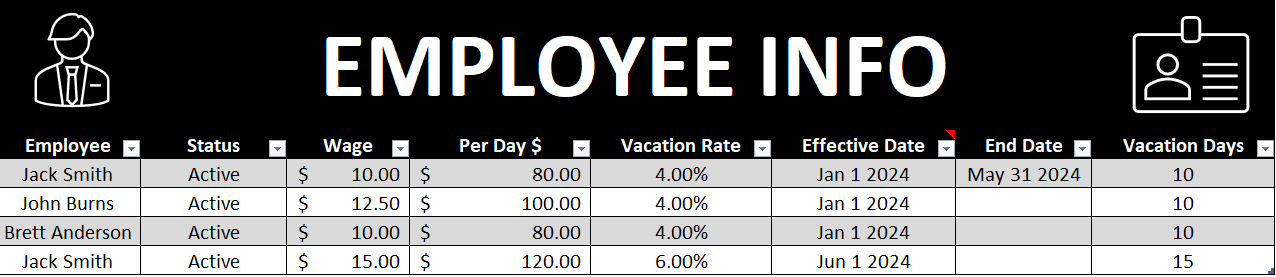
The first tab is the EmployeeInfo tab which is where you will need to enter your employee information. The Per Day $ and Vacation Rate fields are automatically calculated. Everything else, you’ll need to enter in. In the below example I’ve filled in some sample employee information:

Vacation accrual template showing Employee Info information.

You can replace the data in the table and you can also add rows by just typing the employee name in the next blank row in column A and the table will automatically re-size.

If you do not want to track dollars accrued then you can simply leave the wage field blank. This template will allow you to track vacation dollars and hours even if there are wage or vacation rate changes. In the above example, Jack Smith had a wage of $10 from January 1 until May 31. And from June 1st his wage changed to $15 and vacation rate increased from 4% to 6%. I’ll go over this calculation later in this post to show you that it has calculated properly in the reconciliation tab.

If there are no rate changes you can leave the end date field blank. You only need to use the end date field if the employee has a change in vacation days or wages, or is no longer with the company. In the latter case you will also want to set their status to Inactive. Doing so will exclude them from the JE tab and calculation.

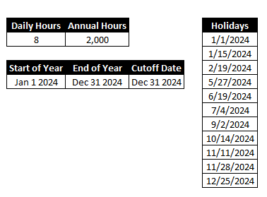
The next section is to ensure the calculation is done correctly and the right percentages are used – daily hours will likely stay as 8 and the annual hours to used in the vacation rate calculation. So if you are paying an employee 4% vacation that is equivalent to 10 vacation days based on 2,000 hours.

Also on this tab is a section to enter the holidays for the year, and this is to ensure that the vacation calculation ignores these non-working days.

The cutoff date is up to what date you want to reconcile to. So if you wanted to know what the vacation liability looks like at the end of the year you would set it to Dec 31, as I have below.

Vacation template with fields for holidays, daily hours, and date cutoffs.

The next tab is the TimeOff tab. This is where you can select when the employee took vacation, and I added an option for sick as well in case you wanted to track that as well.

Time off tab in the vacation tracker template.

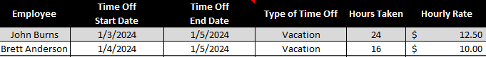
In the above example, John Burns is away January 3rd, 4th, and 5th, so I enter the 3rd as the start date, and the 5th as the end date. The next business day would be the day he is back at work. The hours taken reflects the average daily hours from the previous tab. The wage information also comes from that tab.

On the Calendar tab you will see a year-long calendar off the time off. This isn’t part of the vacation calculation but allows you to visually track vacation and sick time taken.

Chart showing days when an employee is off work.

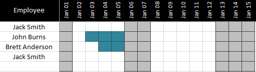
You see above that the days for January 3,4, and 5 are highlighted for John Burns to indicate he took vacation on these days. Sick days will show in a different colour. Weekends and holidays are also filled in with light grey. This would be more of a scheduling tool when you are dealing with many employees and wanted to minimize time off conflicts and overlaps.

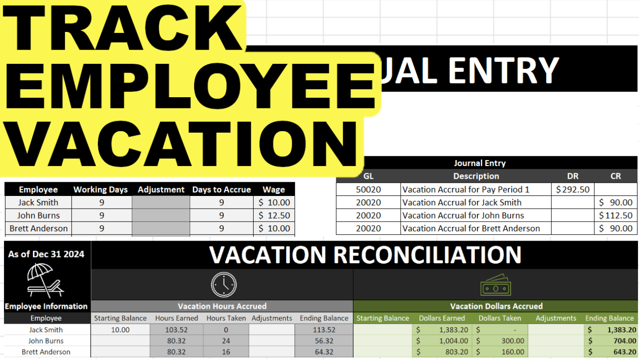
The Reconciliation tab shows a summary of all of the time earned and vacation time taken off.

Vacation reconciliation showing vacation hours accrued.

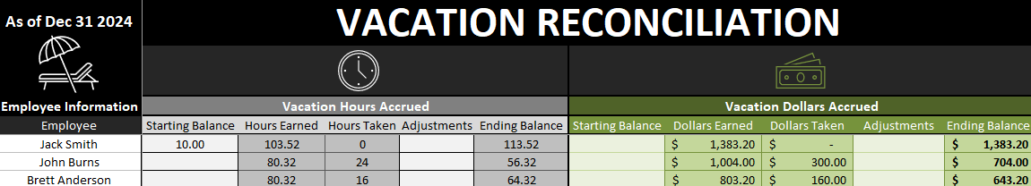
You can enter a starting balance if you carry forward vacation from the previous year, and adjustments for any items not captured in the hours earned or time off taken (e.g. vacation pay out). The other cells are formulas and should not be modified.

Verifying the Vacation Reconciliation Calculations

I will refer to my example above where Jack Smith had a change in wage and vacation rate. His wage won’t affect this calculation but his vacation rate will.

From January 1 to May 31 he will accrue at a rate of 4%. Since he works 8 hours a day x 106 working days which fall within this range once holidays are factored in, that is a total of 848 working hours. 4% of this total is 33.92 vacation hours.

The second range is from June 1 until the end of the year (you can adjust the cut-off date in the EmployeeInfo tab). During this range there are 145 working days x 8 hours for a total of 1,160 total hours worked. At his new rate of 6% this is 69.60.

If I total 33.92and 69.60 that gives me 103.52 hours earned which is what the reconciliation shows.

If you track dollars there is a separate section for the dollars accrued which works in the same way.

Again, going back to my example earlier, Jack Smith had a $10 wage from January 1 to May 31st at a 4% vacation rate. If I multiply 106 working days by his daily pay (daily hours of 8 x wage of $10 = $80 per day) then I arrive at 106 x 80 = $8,480. And 4% of this is $339.20.

Now from June 1st to Dec 31st that is 145 working days x his new daily rate of $120 ($15 wage x 8 daily hours) is a total wage of 17,400. And 6% of 17,400 is $1,044.00.

If I add the two amounts together, I get $1,383.20 (1,044.00 + 339.20). As you see this equals the dollars earned for Jack Smith.

Vacation Accrual Journal Entry

The last tab is the JE tab which is used to generate your vacation accrual journal entry.

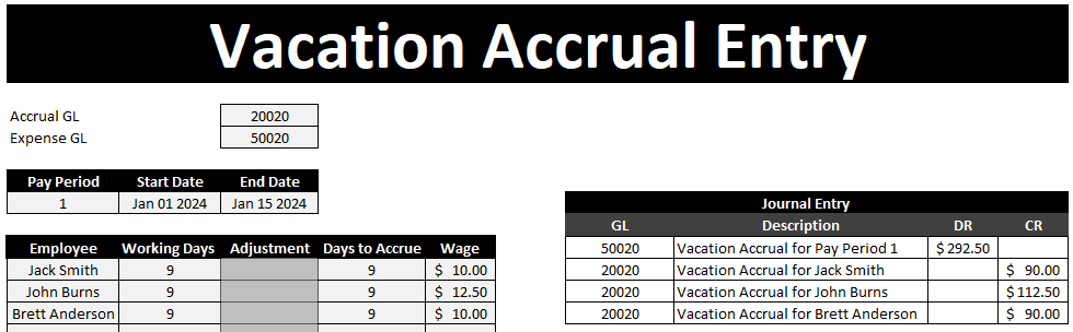
You will need to specify the GL accounts, pay period, start, and end dates. There is also a space where you can put an adjustment for an employee. For instance, your accrual might be for a two week period but if someone was terminated or shouldn’t have accrued for any period of time here is where you can make the adjustment.

The employees listed as active will show up in this list as well as their wage during the dates you enter – as long as you don’t have rate changes that occur in the middle of a pay period there should be no issues here.

Please note this spreadsheet should be used to help reconcile to your payroll provider’s data to ensure accuracy and completeness. Do not use this spreadsheet alone in determining your vacation liabilities as I do not offer any guarantees as to its accuracy.

Download the Vacation Accrual Template

Free version: Download Here. The free version is limited to 4 spots for employees on the EmployeeInfo tab and the sheets are locked and there is an ad in the Excel ribbon.

For the full version (no ads, locks, or limits to # of employees) click on the following button:

Get the Full Version

NHL Playoff Tree 2021: Prediction Template

March 25, 2017

by admin with No Comment predictions template

Standings updated as of May 14.

The NHL playoffs are coming soon and so I have set up a template for predictions that you can use.

Download Template

It is fairly straightforward – you select the team you expect to win in each bracket and the number of games. The page can print out easily into one page but the results are also stored in a more data-friendly version in the Results tab.

On the standings tab is where you will find the seeding of the playoff teams. This is important for the purpose of re-seeding the teams that remain in the semifinals.

Once you get to the semifinals, make sure to click the Re-Seed Semifinals button so that the correct opponents are facing each other. If you want to start over, click on the Reset Selections button.

Bank Reconciliation Template: Automate and Easily Reconcile Transactions

March 22, 2017

by admin with 3 Comments bank reconciliation template vba

PLEASE NOTE THERE IS A NEWER VERSION OF THIS TEMPLATE AVAILABLE HERE

A bank reconciliation can be a time-consuming process but this template can help speed it up. By assigning categories and setup quick ways to match items, you can quickly accelerate the reconciliation process. With an easy interface to match transactions, this template should help speed up what can otherwise be a tedious process.

Download Options

This version has been discontinued. Instead, please refer either to the 2020 or 2023 versions.

Note on #NAME? Errors

If you see this error message in the spreadsheet it means you have not enabled macros when opening the file or the calculations have not been able to update. If you think macros have been enabled and updated calculations but don’t see the results updated, then just try re-opening the file and that should fix the issue.

How to Use This Template

This template allows you to easily reconcile your bank to your book by 1) categorizing transactions, and 2) reconciling any matches based on those categories.

Setting up Categories to Match Transactions

In order to categorize transactions, you will need to use the Setup tab to first create the rules that will find and identify categories. The setup tab has five columns: Category, Identifier, Key, Length of Key, and Gap.

The Category column is simply the name of the category (e.g. wire transfers, deposits, cheques).

The Identifier is what needs to be in your transaction description to be flagged as belonging to this category. For example, suppose the following description on your bank statement indicates cheque # 1234 was cashed:

C#1234

In the above example you would want to set C# as your identifier since that is how you can identify this is a cheque and should belong to the cheque category. The category can have multiple rules (for example, the way a cheque is indicated on your bank is likely not the same as on your general ledger)

The next column, the Key, is what should be used to try and match and reconcile these types of transactions. This is a drop-down selection as there are multiple options: use date, use letters after identifier, use numbers after identifier, and use alphanumeric string after identifier. You can also leave this blank if you don’t want the template to try and automatically reconcile these transactions or if there is no discernible key that can help identify the transaction.

To use the date will mean just the date is used, nothing else. In the case of a cheque this will not work since you might have multiple cheques deposited in a single day, so to just look at date will not correctly reconcile these types of transactions.

In the case of cheques you will want to select ‘Use numbers after identifier’ since that will pull only numbers and not any text. If you need text you can select the option for ‘Use letters after identifier’, or if you need both numbers and letters – ‘Use alphanumeric string after identifier’

The Length of Key column is how long you want the key to be. Suppose the following description:

C#12340000000

Although the cheque number is 1234 the description leaves trailing numbers afterward or might have some other detail afterward that doesn’t pertain to the cheque number. In this case you will not want every number, but just the first four.

The Gap column is used if you don’t want to start retrieving text or numbers after the identifier. For example:

C#001234

In the above example there are two zeros before the cheque number. In such a situation I would set the gap to 2. This would skip the first two characters after the identifier and then start pulling numbers or text after that.

In my example image above I set the identifier to C#, a key length of 4, and a gap of 2. Here is some sample data and how it extracts the key field based on the rules I set out above:

In the first row there was no space between the identifier and the cheque number, as a result, my key only pulled the last two numbers.

In the second row there was one space, so only three numbers were pulled.

In the third row there were two spaces and as a result all four numbers were correctly extracted into the key field.

In the fourth row I added trailing 0s after the cheque number but since my length is set to 4, it does not include those extra numbers.

In the fifth and six rows I show that whether it is numbers or letters before the cheque number is irrelevant since the gap is set to 2. Now in the case of row six, I would not need to set a gap because if I am only looking at numbers it would have skipped the letters anyway.

Note that these rules are not specific to either the book or bank tabs; any rules will be applied to both. However, in all likelihood you would need to setup rules for the same type of transaction multiple times since the way your book shows a type of transaction is probably not the same way your bank will.

If for whatever reason there is no consistency in how some of your transactions appear you could leave the details on the setup tab for the key as blank, that way you still can categorize the transactions (if there is an Identifier) but with nothing set for the key the template won’t match any of those transactions for you, which brings me to the next part: reconciling the data.

Matching Transactions

In order to reconcile that data you will of course need to download your transaction details into the ‘Bank’ and ‘Book’ tabs. Columns A:D are highlighted in yellow and those are the only ones you need to fill in. They include fields for Date, Description, Debit, and Credit. The Description field is the field that will be used for finding what category a transaction belongs to and extracting the key.

Columns E:H are formulas and are pulled from columns A:D.

In order for the template to match and reconcile items, it will look at the following:
– Are the categories the same?
– Do the keys match?
– Do the amounts match?

If all three criteria match, then the Status column will show a ‘-‘ indicating 0; that the amounts are reconciled. Otherwise it will show a value of ‘O/S’

There is also column I, Manual Override. If you mark an ‘X’ in this field, it will make transaction marked as reconciled, regardless of whether the template finds a match or not.

In the above screenshot the second row is reconciled once I enter an ‘X’ in the Manual Override column. Any reconciled items will highlight in green.

Alternative, you you can select a line item that has a status of O/S and click CTRL+SHIFT+X which will bring up the Reconciler window which will show you potential matches for the item you are looking to reconcile.

In the above example I pressed the shortcut keys while selecting the row with the $5,000 wire transfer. Since it is O/S it pulls up the Reconciler window. The Reconciler shows all the wire transfers from both the previous O/S tab as well as the Bank tab (in this example I was on the Book tab). Exact dollar matches show up at the top. Note the first result shows an amount of -$5,000 – the negative does not indicate a credit, it pulls the amount from the amount field which just shows the negative as being an outflow of cash. Because an outflow of cash on the bank is a debit, if I select the -$5,000 it will show $5,000 DR as being the amount matched, which is shown on the next screen:

Because the debits match the credits, the Match Selections button has turned green and can now be pressed. Doing so will enter an ‘X’ in the manual override field for these amounts. You will only be able to match the selections if the debits and credits match. You can select multiple items if they add up to the total outstanding.

Completing the Bank Reconciliation

Once all the bank and book data are entered and you have finished matching which items you can, go to the Reconciliation tab where there you will see three buttons on the right hand side:

The Reconcile button will generate the reconciliation and show you which items are outstanding. It will group the outstanding items by category – refer to the screenshot at the beginning of the post. If the adjusted balances match and the amounts reconcile to 0 then it will highlight that line in green, otherwise it will be in red to indicate a variance. The reconciliation date you will need to enter in the yellow highlighted cell.

The New Month data will clear all your existing data but before doing so will put your existing O/S items into the Previous OS Items tab so on your next month’s reconciliation they can be used to match new transactions.

For example, if cheque #1111 does not clear this month it will be moved to that tab. If on next month’s transactions there is a transaction on the bank for this cheque number the template will be able to reconcile it automatically. Nothing extra needs to be done to do this, as when looking for matches, both the bank and book tabs look at the Previous OS Items tab to clear any items from there as well.

Lastly, the Clear Data button will do just that – get rid of everything from every tab.

The template at the top has some sample data so you can test out and see how it works.

Use Excel’s Random Number Generators to Populate Sample Data

March 16, 2017

by admin with No Comment index intermediate rand randbetween random

Excel has random number generator functions which are useful if you need to test a template or create some sample / dummy data.

The RAND function returns a number between 0 and 1. You could multiply this by a factor of 10 or 100 to get a much larger number if you need it. Once you are happy with the data that has been populated then you will want to copy and paste it as values otherwise the numbers will change every time a recalculation occurs. This is true of any random number function in Excel.

Similarly, the RANDBETWEEN function will return a random number between a range that you specify. In the below example I use 1 and 100:

If I used the RAND function and just multiplied by 100 I could get similar results to RANDBETWEEN. The latter just saves you that extra step by being able to specify your parameters right in the formula. It allows you also to be more specific (say for example I wanted a random number between 1 and 35, the RANDBETWEEN function would certainly be easier to use)

If you do not like the random numbers you have generated, you can simply just hit the delete key on an empty cell and your random numbers will be regenerated. If you don’t want your numbers to change anymore then you will want to copy them and paste as values.

To use this to create sample data I am going to make two lists, one for employees, one for stores. From there, I can use the RANDBETWEEN function in conjunction with the INDEX function to extract values from the lists:

In columns A and B I am just using the RANDBETWEEN function to select a number between 1 and 5, as that is the number of different employees and stores I have listed in columns C and D. In columns E and F I use the INDEX function to extract from those lists using the random numbers generated in columns A and B.

I will break down the INDEX formula in column E a little bit here:

=INDEX($C$2:$C$6

In the first argument I am selecting my employee list since this is where I want the result to come from. I also lock the cells using the $ sign to ensure that as I copy the formula down that range is locked and will always reference C2:C6.

=INDEX($C$2:$C$6,A3

The second argument in the INDEX function is the row number from where I want to pull my value. Cell A3 is my first random value – which in this case is 4. This means that from the Employee List range (C2:C6) I want the value on the fourth row of that range – which is not row 4, it is row 5 since I start counting from the start of the range, which is on row 2. As I copy this formula down the row number will change to the corresponding value in column A.

Because the lists only have one column you could actually stop here.

=INDEX($C$2:$C$6,A3, 1)

The last argument in the INDEX function is the column number. In this example I only have 1 column in my lists so the value is equal to 1. You could skip this argument and it will still work however it’s good habit to always enter the column number.

The above formula tells me to look at range C2:C6, and extract the value from the row that is referenced on A3 (which is 4), and from column 1. That point of intersection is Employee 4, since it is on the fourth line of that range, and in the first and only column.

If I copy the formula down a cell it will do the same except this time pull the value from the row referenced in cell A4 – this time it is 2. As a result, my result is Employee 2 since that value is on the second row of the range and again in the first column.

Column F is the same formula as column E except this time it references the store list (column D) and the second RANDBETWEEN column (column B). This is just to show you how you might fill in multiple items. You wouldn’t want to use column A again otherwise you are guaranteed that the same row will be returned and you will always have Employee 4 tied to Store 4, and thus, not truly random combinations.

In this example I have my lists, random numbers, and results all in the same area for illustrative purposes but they do not need to be even on the same sheet.

How to Use Goal Seek in Excel

March 7, 2017

by admin with No Comment goalseek intermediate tips & tricks

Excel’s what-if-analysis options aren’t the greatest, but one option which is very useful and can save time is Goal Seek. What Goal Seek effectively does is it can do trial and error for you in seconds, and be much more precise than doing it manually.

In many examples you could use algebra to get to your answer but if it’s a one-time calculation perhaps it’s not worth the trouble of going that route. For example, suppose I had an investment of $1,234 and wanted to know what average return would be needed for it to grow to $10,000 after 10 years. This can certainly be done with algebra, but Goal Seek can also do it. Below, I have entered my inputs in yellow.

My ending balance is equal to the following formula : =C4*(1+C5)^C6

C4 = Investment

C5 = Required Rate of Return

C6 = Years

Next, I will select Goal Seek from the Data tab under What-If Analysis

The next screen prompts me to enter which cell I want to set to which value, and which cell I want changed to accomplish this (the variable). In my example I use C7 for the set cell box (this is my desired ending balance), the value is 10,000, and by changing cell I enter my required rate of return (which is C5).

After clicking OK it fills in the required rate of return as 0.23273147. It also sets the value in C5 to this amount as well. If I hit OK on the next screen the value in C5 will keep this value, if I cancel, it will revert to what was there before – nothing.

This was a simple example but there are also more complex ones it can be used for. Another example could be an amortization table. The table below has a principal amount owing of 10,000, an interest rate of 5%, a payment of 550 per month. This is what it looks like:

So it will take roughly 19 payments to for this amount to be paid off under the terms described. But let’s say I wanted to know precisely what interest rate would have to be applied to make the ending balance at payment number 20 equal 0. I don’t want an extra payment for the balance to be included at the end, just so that it perfectly matches 0 after payment 20.

To do this, I go back to Goal Seek. For the first box (set cell) which is what I want my result to be – I select the ending balance at payment 20 – currently it is (579.34). This is cell F27 on my spreadsheet. The second box is what result I want, which in this case is 0. Lastly, my variable, or the cell I want changed to make this work – that is my interest rate, which is in cell C4 – currently it is at 5%. These are what my inputs look like:

Once I hit OK, I get the following:

You’ll notice now my target value matches my current value and the Goal Seek was successful. It has changed my interest rate to 11% – not exactly 11%, 11.1048262490731%. A very precise percentage that has allowed my table to reach 0.

Goal Seek can be used in a variety of different circumstances as you can see. As long as you have a formula like in the above two cases that the change cell (e.g. variable) directly effects, then it should work. I could have selected the payment as my change cell rather than the interest rate and my result would be as follows:

It would indicate a rounded payment of 522.16 (exact amount of 522.162995552194) would be needed to pay off after 20 payments with the interest rate staying at 5%.

The one limitation of Goal Seek is that you can only use one variable. But beyond that it does it very well and can help save you a lot of time.

Calculating Date Differences Using VBA

February 26, 2017

by admin with No Comment dates functions vba

In VBA there is a custom DateDiff function that allows you to easily calculate the difference between dates – whether you want the difference to be in days, weeks, months, years, it is easier to accomplish this in VBA than through regular Excel formulas. I have piggy-backed off the DateDiff function to make a custom function in Excel that makes it easy to use as a formula in your spreadsheet.

The custom function I have created is called datecalculation and consists of three arguments: start date, end date, and interval. The interval determines how the difference is calculated. The interval needs to be in quotations and use one of the following codes:

Below is an example of how the function work when computing the difference between January 1, 2016 (cell C2) and January 1, 2017 (cell C3). The interval codes are in column A.The result column is the date difference according to the selected interval.

To make this function work in your spreadsheet simply insert the following VBA code. If you are not sure how to do that, please refer to this post, specifically the section about inserting VBA code.

————————————————————————————————————————

Function datecalculation(date1 As Date, date2 As Date, interval As String)

datecalculation = DateDiff(interval, date1, date2)

End Function

————————————————————————————————————————

Incrementing dates by month using a formula vs autofill.

How to Do Date Calculations in Excel (and Format Them)

February 19, 2017

by admin with 3 Comments dates intermediate

In this post, I am going to cover some commonly used date functions and show you how to do some basic date calculations in Excel.

Incrementing Dates by Days and Months

One of the more common date calculations in Excel is to increment your dates. If you want to increment a date by months, years, or days, then you can use the DATE function to do so. This function has three arguments: year, month, and date. If I have a date in cell C3 and I want to make cell C4 one month later, I would use the following formula:

=DATE(YEAR(C3),MONTH(C3)+1,DAY(C3))

For each of the year, month, and day arguments I used their individual functions. The YEAR function will take the year of the date specified, as the MONTH function will take the month, and the DAY function will take the specific day. For the DAY and YEAR functions I simply just referenced cell C3 since I want those values to remain the same. The MONTH function also took the same value from cell C3, however, I added +1 to it as well to increment the value by one month.

If I want to just increment by day, then I can just enter a starting date and drag that value down, and Excel’s autofill will automatically increment the values by one day. Here’s a comparison of the daily increment (where no formula is necessary) and the monthly increment, where I use the formula noted above:

Now, there is another way, an even simpler way, just by using Excel’s autofill feature that I can increment by month. If I enter my starting date in cell B3 and pull it down using the fill handle, Excel will increment by day. However, if I select cell B3 and pull down the fill handle while also holding down the right-click button, it gives me the option to select how I want to increment – including fill days, weekdays, months, and years.

This way you can ensure Excel increments as you like. If you just use the fill handle without the right-click button you don’t get these options and Excel fills in the data how it thinks makes sense. Interesting to note that if you fill in cell B4 with the next month, and then select cells B3:B4 and then use the fill handle, then Excel has figured out you want to increment by months and doesn’t increment by days anymore. The more of a pattern you show Excel, the more likely it will know what you are trying to do.

In the above picture if I now double click the fill handle my daily increment will become monthly since I have selected two points in my series. And since the two points have a monthly interval, Excel assumes I want the rest of the series to also have monthly intervals as well. The result becomes this:

You may wonder what the point would be of using the date function in the formula above if you can just use the fill handle since it is faster and easier. The main benefit of using a formula is if you don’t want to have to use the fill handle all the time. If you just need to set up your dates one time, then certainly the fill handle makes sense. But if you are working with a large data set that you will continually add to, you might find it a bit easier to have a formula there as opposed to using the fill handle each time and making sure it is incrementing correctly.

Calculating the Difference From/To Today

If you want to include today’s date in your calculations, you can use the TODAY() or NOW()functions. These functions have no arguments and you just enter them with both parentheses. This will generate today’s date. The difference between the two functions is the NOW() function also includes the time. But for the purpose of calculating the difference in days, either one will do the job.

Alternatively, you can use the shortcut CTRL+; which will plug in today’s date. If you want the date to update every time you open the spreadsheet then you are better off using the functions. If you want to do a one-time insertion of the current date never to change later, then the shortcut will do. It is no different than just entering the date yourself.

End of Month Calculations

Suppose I wanted to not calculate the number of days from today, but the end of the month. What I could use is the EOMONTH function. This has two arguments – start date, and months. If I wanted to use the end of the current month, I would enter the following formula:

=EOMONTH(TODAY(),0)

If I wanted the end of next month, then I would change the 0 to a 1:

=EOMONTH(TODAY(),1)

The months argument just tells Excel how many months ahead to go. Whether you change the months argument or alter the start date to get to a later month end value, it doesn’t matter, both methods can get you to the desired result.

Calculating Workdays

Up until now, I’ve gone over how to calculate the difference in days. But suppose I wanted to calculate only working days. To do this you can use the NETWORKDAYS function which will take the starting date, ending date, and calculate how many workdays fall in between. To be more accurate you could also include a list of holidays into the function (which you will have to populate).

In the above example, I selected Jan 2 and 3rd as holidays so as a result, the NETWORKDAYS function with holidays has two days fewer than the function without holidays since those days both fall within the date range. Without a list of holidays, the NETWORKDAYS function effectively calculates weekdays since it would only ignore weekends. Also note that in the argument for holidays, do not include any text fields such as a header for holidays. If my range included the header then it would return a #VALUE error.

A similar function, WORKDAY takes the starting date, and you select how many workdays you want to advance by, and it will return a date result for the next working day after the days you specified. Again, you can list the holidays to ensure a more accurate calculation.

If you don’t use holidays then both functions (NETWORKDAYS and WORKDAY) will not adjust for them. However, both functions will recognize and skip over weekends and so if you leave holidays blank they effectively just look at every weekday.

Calculating Weeks, Months, Years

If I wanted to do date calculations in Excel to show the difference between two dates in weeks, what I could do is use the WEEKNUM function and then use my date as the argument for that function. Once I calculate this for both dates then I just calculate the difference. This strictly looks at the week of the year, so it won’t take into account whether one date is a Friday and the other a Monday.

And if you wanted to you would be better off dividing the difference in dates by 7 to get fractional weeks.

For months you can do the same thing, except using the MONTH function which will yield a result from 1 to 12. The YEAR function will do the same as the month function, give you the year of the specified date, which you then can use in your calculations to calculate the change in years. You can also use the YEARFRAC function if you wanted to calculate the difference in fractions of a year, to give you a more specific result when calculating the difference in years.

Formatting Dates

In addition to just doing date calculations in Excel, it’s important that your dates are also formatted properly. You can format dates so they display exactly how you like right through the format cells option. The easiest way to do that is to go to the cell formatting (right-click format cells, or click ctrl+1), and select the CUSTOM category.

If you want month/day/year (which it may already be set to) the formatting is just m/d/yyyy. But what if I didn’t want to show all four numbers for the year, just the last two? Then I would set it to m/d/yy. You can flip the d and the m around so it is d/m instead of m/d and then you have day/month/year. If you use two d’s rather than one you will get a 0 if you are in single digits for the day. For instance, instead of 1/1, you could get 01/01. You will notice the changes in the sample box above as you change your custom category.

Here is a quick summary of the use of letters and what results they will yield:

m or d: will use 1, 2, 3, etc.
dd or mm: will use 01, 02, 03, etc.
ddd or mmm: will spell out the abbreviation (e.g. ‘Mon’ for Monday, or ‘Nov’ for November)
dddd or mmmm: will spell out the entire day or month (e.g. Monday, November)
y or yy: will use the last two digits of the year.
yyy or anything more: will use the full four digits of the year.

If I wanted to use a formal date that showed the day and month spelled out, followed by the numerical day, a comma, and the year, I would use the following format:

dddd mmmm d, yyy

If you liked this post on How to Do Date Calculations in Excel (and Format Them), please give this site a like on Facebook and also be sure to check out some of the many templates that we have available for download. You can also follow us on Twitter and YouTube.

Shading Areas on a Chart to Highlight Gaps and Variances

February 5, 2017

by admin with No Comment charts intermediate variances

When comparing forecasted amounts vs actuals one way to help emphasize and highlight variances is by shading those areas. I’ll show you how to easily do that in this post.

Below is my starting data set

I will need to create two extra columns to this data set. The first one I will just call Starting Values and they will match my forecasted amounts. The next column, called Variances will be equal to the actuals less forecasted values.

Next I will plot a line graph with these values.

I will need to change the chart type for the starting values and variances data sets. They need to be set to the stacked area charts.

For the starting variances series, click on Format Data Series and under the Fill section select No Fill. What remains are the shaded areas in addition the line graphs. You can change the shading to a different fill colour or texture.

Plotting Vertical and Horizontal Lines in Charts

January 27, 2017

by admin with No Comment charts intermediate

When charting something on Excel you sometimes may want to add vertical lines to identify key dates, or horizontal lines for target or benchmark amounts. In this post I’ll show you how to do both.

Horizontal lines can be used to identify target or benchmark amounts while vertical lines are useful to mark dates. In my example I’ve downloaded googles historical closing stock prices for the year and I’m going to mark the year long average and identify their earnings dates

Horizontal Lines

I’ll first start with horizontal lines. If you have amounts on the y-axis then a horizontal line can act as an indicator to show if the amounts have crossed a targeted amount. In order to add a horizontal line all you’ll need to do is create another column in your table.

The key thing for this column is all the values have to be identical for each entry. I can set it to a single number and copy it down, or I can do a calculation as well. What I will use is the closing price average in this column using the AVERAGE formula. If I copy this down I am left with a value that stays constant for the entire data set.

If I chart this graph using a line chart my horizontal line is now visible

Vertical Lines

Vertical lines are a bit more tricky but not difficult. In my example I am going to put a vertical line at every earnings date since I know those days will have a lot of fluctuations and will also create quarterly intervals. I have created a column for all the earnings dates in the year, aka my earnings calendar.

Again I will need to create another column in my table.

In this column I will look to see if the date for this row matches one of the dates in my earnings calendar. If there is a match, I will set the value to 1. Whether you use the MATCH formula or the VLOOKUP formula doesn’t matter. But I will use the MATCH formula in this example. The key is including the IF and ISERROR formulas because if I do not find a value it will return an error, and specifically I will use the NA() formula to return the NA error so that that amount does not appear on the chart as a zero. And if it is a match, I can make it set to 1.

First I will start with the IF function, add ISERROR, and add the MATCH function to now see if the date on this row matches anything in my earnings calendar), and if it is not a match, make it equal to an NA error, otherwise make it equal to 1 indicate a match.

My formula looks like this:

=IF(ISERROR(MATCH(A2,G:G,0)),NA(),1)

Where column G is where my earnings calendar is located.

Now I will copy my formula all the way down. It may not look terribly nice in your table with all those errors but it will get the job done.

I’m ready to chart my graph now. Select line chart again. However unlike for the horizontal line, it needs some work.

The earnings dates need to be plotted against the secondary axis. To do this, I right click on the series and click Format Data Series and select Secondary Axis.

Next, I need to change the series chart type so that it is a column chart. I will right click on the series again and select Change Series Chart Type and then select a column chart.

I will go back to format the data series once more to add a border which will allow me to make the line look thicker. By going to Border Colors this time I can specify the colour, and then under Border Styles I can modify the Weight.

I will now format the secondary data axis. I will set the maximum height equal to 1, the value that I set for the earnings column when there was a match. It doesn’t matter what you set that value to, whether it is 1, 100, 1000, you will just need to change the axis accordingly to make sure that value is at least as large as your scale to have the line go all the way across. If you have values that you are currently using on your secondary axis you will want to take that into account and consider what is a good maximum value for that secondary chart, and use that value, rather than 1.

Next, I will hide the secondary axis (if you need it for other values obviously this is optional). To do this right click on the axis, click Format Axis, and set Axis Labelsto None.

Now my chart is good to go with both vertical and horizontal lines.

Create a Customer Cover Letter with my Form Letter Template

January 11, 2017

by admin with No Comment letter template vba

Download Template

This template allows you to create a customized letter – be it a cover letter or any other kind of letter from a pre-defined list of sentences and paragraphs that can also utilize variables. In order to accomplish this you will first have to setup the sentences, paragraphs, and variables you will want to use. But once you have done so you can easily reuse them going forward.

Setting Up Variables and Paragraphs

In my template I have two sections – one for variables, and one for paragraphs. In the variables section you can setup variables that can be used in your content. These will be values that will likely change from one letter to the next. In my example I have a % sign in front of the variable name. The purpose for this is to make it easier to accurately identify where a variable has been used. However you don’t need to use it, but you would want to ensure your variable name is unique and not a word that you might use in your content that you don’t intend to use as a variable.

In the paragraphs section here you can setup sentences or entire paragraphs that you would potentially like to add to your letter. The title is just a way to identify the content, the paragraph is which paragraph the content relates to. For example, I have multiple titles that relate to the paragraph called experience.

This means that if I add all of these items, they will be stitched together to form only one paragraph. This is just to help organize my paragraphs to make sure I don’t have a paragraph for each item I want to add. You may not have enough to write a paragraph about each skill set you have, but instead you may want to add it on to a paragraph that relates to the content.

If I look at the title labeled ‘Introduction’ this has a related paragraph by the same name. There are no other items that relate to the introduction paragraph. So this means if I add the Introduction, it will be an entire paragraph on its own, and no other items I add will be added to it. The Introduction also has all three variables I setup – %HIRINGMANAGER, %POSITION, and %COMPANY. These are all variables that you would expect to change from one cover letter to the next. I can certainly use more variables and put them into other content but in this example I only did it in the Introduction.

If you need to add more rows you certainly can do that, as well as changing the existing content, titles, and related paragraphs. If you want to add lines within a cell, all you have to do is when you are editing in the cell click ALT+Enter and you will create an additional line of text within that cell. This will allow you to help space out your descriptions as you wish.

Updating Variables

Once your paragraphs and variables are setup, click on the Create Letter button. You will first be prompted to enter values for your variables. Here I will update the name of the hiring manager I’m applying to, the name of the company, and position.

Once done, click Update Variables.

Finalizing the Letter

Next, you can select the content you wish to add to your letter. The titles will appear in the drop down boxes. Go from top to bottom. As you select an item it will be added to your letter.

When I add Introduction my variables are now updated to reflect what I entered at the earlier screen. You can also edit the letter in the preview box.

However should you make any changes to the drop downs your edits will be gone. So make sure to do edits only after you’ve selected all the content you wish to use.

Once you are done, click on the Copy to Clipboard button and you can now paste it into a word processing document, email, or wherever you like.