Many people are out buying homes this year as interest rates are at record lows. But figuring out what you can afford can sometimes be a bit challenging. You need to factor in how much of a downpayment you can afford, what your monthly payments will be, and your income. Oftentimes you’ll end up doing multiple what-if scenarios. However, with the free mortgage payment calculator in Excel, you can get a quick snapshot of all the pertinent information to help you determine which house prices are within your range. You can download the template here.
How the calculator works
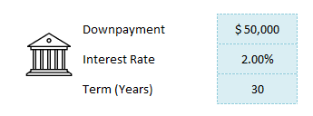
There are three sets of inputs on the calculator. The first section relates to the mortgage itself — how much of a downpayment you can make, the interest rate that’s available to you today, and how many years long your mortgage will be.
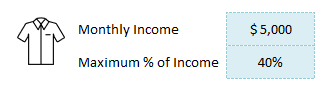
The second section relates to how much income you make as well as how much of your income you want going to cover your mortgage. This is a good way to gauge affordability to ensure that the monthly mortgage payment is within your means. For the monthly income, you’ll want to use after-tax income since this is what will actually be available to you to pay your mortgage payments and other expenses. This is also tied to the worksheet’s conditional formatting. When the % of the monthly mortgage rises above your maximum%, the cells will highlight in red to show that these house prices will be too expensive based on your threshold.
This is an optional section and if you don’t enter it then the spreadsheet simply won’t populate the % of monthly income and there won’t be any conditional formatting applied.
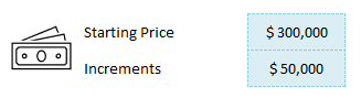
The last section is simply what house price you want to start at, the minimum value that you want to look at. There’s also an area where you can determine at what increments each option should increase by. For instance, if you want to look at a very narrow range, you might put $10,000 to see the different scenarios if the house price increased by $10,000. If you’re looking at a much wider range, you could increment the values by more, such as $50,000 or $100,000.
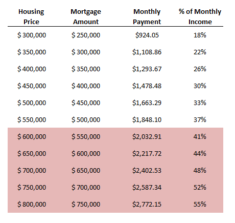
As you enter values in these fields, the mortgage payment calculator will update its results and show you how the different scenarios look like at the different prices.
The above table will be updated immediately as you make changes to your inputs. Please note the spreadsheet is locked and you only can enter data in the inputs. This is to prevent user error and the possibility that formulas are overwritten.
If you liked this post on the mortgage payment calculator in Excel, please give this site a like on Facebook and also be sure to check out some of the many templates that we have available for download. You can also follow us on Twitter and YouTube.
Last week, I covered how to calculate discounted cash flow. In this post, I’ll build off that worksheet and show you how you can calculate the internal rate of return (IRR) in Excel. IRR tells you the return that you’re making on an investment or project, and at what discount rate the net present value of all the cash flows will be zero. In these scenarios, there’s typically an outlay of cash, usually at the beginning.
In my previous example, I only looked at cash flows coming in. This time, I’ll look at a scenario where you pay money out at the beginning and generate cash flow in future periods. A common example is paying to upgrade a piece of equipment and then generating cost savings from it for x number of years. Knowing the IRR can tell you if you’re making enough of a return off of the investment and whether you should move forward with it. Using IRR can also be helpful when you’re comparing multiple options to see which one is the best one.
Setting up the spreadsheet
This step is about the same as when setting up the discounted cash flow template. You’ll need to enter the different years, the cash you expect to come in or out, and then calculate back what the present value is today.
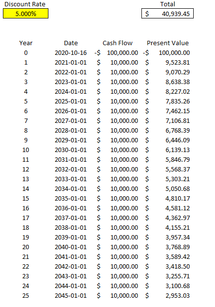
Here’s what the file looks like setting in a scenario where you pay $100,000 upfront and then generate $10,000 in cash flow for 25 years. At a 5% discount rate, in this example the present value of all that cash flow is a positive $40,939.45:
Calculating the IRR
The problem here is the discount rate can be difficult to determine, and that can have a significant impact on your overall returns. And so rather than worry about what your discount rate should be, you only need to determine the IRR — which is to say at what point would your present value be worth $0? If you need a higher return than the IRR the project would be a no-go but if you’re okay with anything up to and including the IRR, then the project or investment would be passable. What it comes down to is the lower the IRR is, the worse the investment is
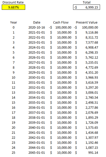
There are a couple of different ways to calculate IRR in Excel. One way is through a formula called XIRR. It only has two required arguments — dates and cash flow. This is why in this example I entered dates for my cash flows rather than just numbering the years. This makes it easier for me to use the XIRR formula. In my spreadsheet, I enter the following formula:
=XIRR(D6:D31,C6:C31)
Column D contains my cash flow and column C contains the dates. Doing this, Excel tells me the IRR is 9.687% for this specific project. But if I work backwards and calculate the net present value, it doesn’t get me right to 0:
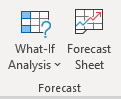
It certainly gets close to 0 and it’s probably close enough that it can help you make a decision about your investment. However, there’s another way to calculate IRR and that’s using Excel’s What-If Analysis. On the Data tab, there’s a drop-down for this option in the Forecast section:
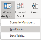
Depending on which version of Excel you’re using, it may show a bit differently, but what you’re ultimately looking for is Goal Seek.
Goal Seek is an accelerated way of doing trial-and-error. Excel’s doing it for you much quicker than you could ever do it by yourself. For IRR, it’s the best solution.
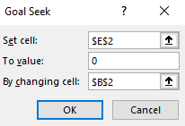
Here’s how it works. You’ll need to enter the cell that you want to get to a certain value, what value that is, and which cell Excel should be changing values in. In my spreadsheet, E2 is where my net present value formula is, and I want that to equal 0. In cell B2 is my discount rate, which is what I want Excel to be changing. Here are what my inputs look like:
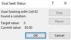
Then, once I click on OK, Excel goes to work. After a few seconds you should see Excel show you that the target value and the current value are a match (e.g. they’re both 0), meaning it’s done its job successfully:
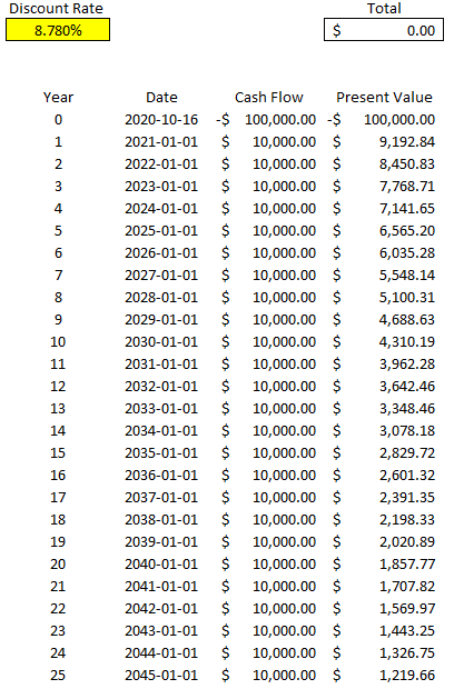
Now, if I look at my template, I see a different discount rate and my total present value is netting out to 0:
As you can see, this is much more accurate than Excel’s XIRR function. You can repeat these steps and make this table for other projects that you can assess side-by-side.
If you’d like to test this out, try downloading the discounted cash flow spreadsheet from my last post and then just using Goal Seek or the XIRR function to determine your IRR. You can remove unnecessary columns from the sheet and then duplicate the table, and then you’ve got a template where you can assess multiple investments against one another.
If you liked this post on how to calculate IRR in Excel, please give this site a like on Facebook and also be sure to check out some of the many templates that we have available for download. You can also follow us on Twitter and YouTube.
Do you need to calculate the present value of future cash flows or assess two options that will impact your cash flow over many years? Excel’s a great place to do that and below I’ll show you how you can easily set up a template to calculate discounted cash flow that you can adjust for changes in the discount rate and cash flow. And if you don’t want to create your own template, you can download mine at the bottom of this post.
In this example, I’ll compare a lump sum lottery win versus a scenario where you receive an annual amount for 25 years. Step one is knowing to calculate present value, which is what I’ll cover next:
Calculating the preset value
To calculate the present value of future cash flow, you need to know what discount rate to use. What you can use is the rate that you can earn on a typical investment. For instance, if you invest in stocks and assume you can make 5% per year, on average, then you might want to use that as your discount rate. If you want to be more conservative, you could use a rate of 2%. Below, you’ll see how the discount rate can play a big impact in your calculations.
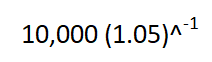
That’s because when calculating today’s present value, you have to use the discount rate to bring the future value back to what it would be worth today. For example, suppose you were to receive a $10,000 payment a year from now, and your discount rate was 5%. An easy way to calculate this is as follows:
You might see other formulas on the web involving fractions to calculate present value but just using a negative power does the trick. This calculation yields a result of $9,523.81. Because you’re not getting the payment today, the value of that money is worth less than the full amount. Consider that if you were to receive $10,000 today and invest it and earn 5%, then a year from now it would be worth $10,500 — more than if you were to receive the $10,000 in a year.
Now, suppose you used a discount rate of just 2%. In that scenario, the $10,000 payment a year from now would be worth $9,803.92 today. Since the discount rate is lower, there’s less of a cost associated with waiting for your payment. If the discount rate was 0%, then there would be no incentive for you to invest your money since a year from now it would still be worth the same value it is today. That’s why when interest rates fall and get closer to zero, people will be less inclined to keep their money at the bank and there’s more demand for gold — since that can be a better way to store wealth at that point.
Creating a template to calculate discounted cash flow in Excel
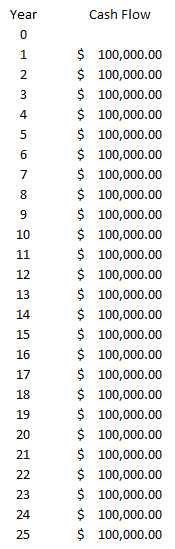
Now that we’ve gone over how to calculate discounted cash flow in Excel, we can set up the template. All that’s really necessary here is to map out the payment schedule, including how much cash you’ll receive every year. Here’s an example scenario of receiving $100,000 for 25 years:
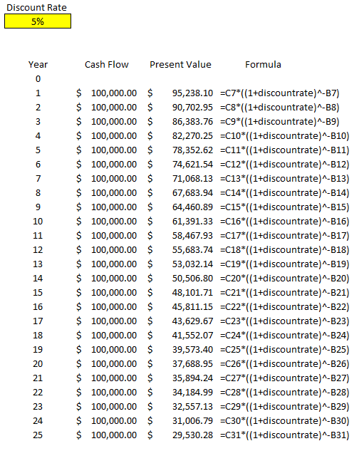
All the payments don’t have to be the same, but for the lottery example, I’m going to keep them that way. What I can do is create another column that will tell me the present value of each one of those payments. To do that, I’ll use a formula that takes the cash flow value, multiples it by the discount rate (I’ll use 5%) raised to a negative power (the year). Here’s how that looks:
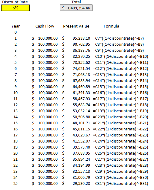
I created a discount rate named range so that it’s easy to reference the percentage and to change it. The only thing left here is to calculate the total of all these payments, to arrive at the present value of all of them:
The total present value of the payments comes in at just over $1.4 million. Even though the total of all the payments over 25 years is $2.5 million, we’re losing a lot of that value because of the time value of money, at a rate of 5% per year.
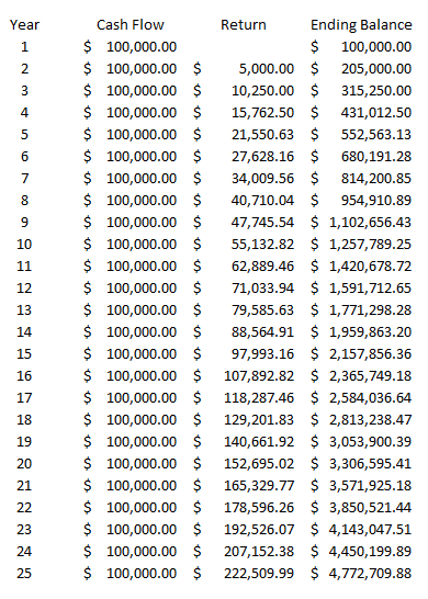
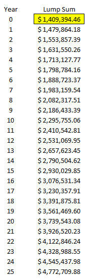
However, let’s prove this out, and to do that let’s look at the future value of all these payments. Let’s assume that these funds will be reinvested and earning a rate of 5% every year. Here’s how much we’d have by the end of year 25:
In this situation, we’re benefitting from compounding and earning 5% on each year’s ending balance, which includes the prior-year return. By the end of year 25, if we were to invest all of these $100,000 payments at a rate of 5%, we’d have a future ending value of $4,772,709.88.
Now, remember, the equivalent of these annual payments is a present value of $1,409,394.46. Let’s assume that rather than receiving annual payments of $100,000, we simply receive a lump sum payment of this and invest it and also earn 5% every year. Here’s how that will look like:
The ending value after 25 years is the same, $4,772,709.88. This tells us that if you’re given the option of 25 annual payments of $100,000 or a lump sum of $1,409,394.46 today, there’s no difference to you (if the discount rate you’re using is 5%). If the discount rate is 2%, then the present value climbs to $1,952,345.65.
As you can see, depending on which discount rate you use, it can have a significant impact on your present value calculations. This template will allow you to quickly change the discount rate and see how the calculation looks under different scenarios. You can also add more years to this calculation by just extending the formulas down. The amounts also don’t need to be identical, they were only set up this way purely for the purpose of comparing lottery winnings in a scenario where you earn one lump sum amount versus equal payments over multiple decades.
If you’d like to download this template to follow along, the free version is available here, which goes up to year 15. For the full and unlocked version, which has no ads and goes up to 30 years, please refer to the product page here.
If you liked this post on how to calculate discounted cash flow in Excel, please give this site a like on Facebook and also be sure to check out some of the many templates that we have available for download. You can also follow us on Twitter and YouTube.
The money spent calculator can help you determine how much a daily, weekly, or monthly recurring expense costs over the course of a year. Simply enter the dollar amount using the slider above and select how frequently you make that purchase. Then, you’ll be given a spending summary by month and by year.
And just for fun, it’ll tell you what that annual spend could’ve translated to if you bought milk, coffee, or toilet paper instead. These numbers are just estimates and will obviously vary by location but they can help illustrate the size of the expense using common items.
If you liked this money spent calculator, please give this site a like on Facebook and also be sure to check out some of the many templates that we have available for download. You can also follow us on Twitter and YouTube.
Several weeks ago, I discovered that Excel had a new function called STOCKHISTORY. It’s able to pull stock prices and a great way to track stock prices and can help calculate returns. Excel does make it clear that it is not for trading purposes. However, it’s still a great way to stay on top of tracks and see how they’re performing. Below, I’ve created a template that will allow you to track stock prices and arrange them from best-to-worst.
Note that for this template to work, you need to have the STOCKHISTORY function on your computer, otherwise you’ll get nothing but errors. So your first step will be to check if it works on your file. Refer to the original post on the function as it will also explain how you can get it on your computer if you don’t already have it. If you’re running on old versions of Excel, you’re out of luck.
But for those that aren’t and that have access to the function, read on.
Entering the ranges that you want the macro to sort.
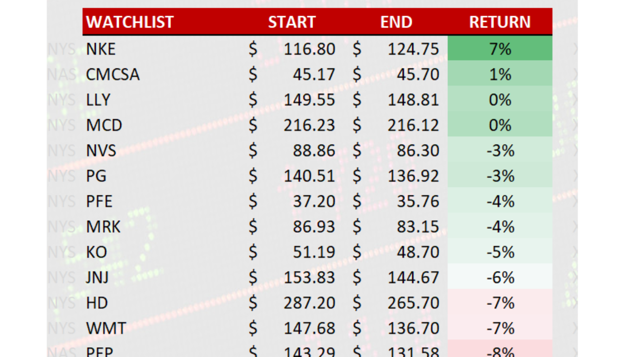
Let’s start with the first one, selecting stocks. I’ve already created three stock sections in this template, which you can of course change. Let’s look at one of them as an example:
The Start, End, and Return values are formulas. The only things you need to enter are the ticker symbols. Off to the left, shaded in light grey, I’ve also entered the code for the exchange. For the New York Stock Exchange, it’s XNYS, while the NASDAQ is XNAS. For a full list of the codes, refer to the original post on the STOCKHISTORY function. If it’s a popular stock that’s on one of the major exchanges, you may not need to enter it. I’ve included the exchange code for the sake of avoiding errors as it’s possible Excel might not know which ticker you’re looking for and select the wrong one.
You can extend the ranges to accommodate more tickers, you’ll just need to copy the formulas down in the Start, End, and Return sections.
Next: the date ranges.
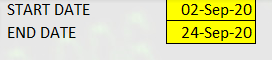
Off to the right of the template, there’s a section where you can enter the start and end dates.
The template will adjust for weekends but not for holidays. If you see a #VALUE! error in the values, that likely means there’s an issue with the date, so you’ll just need to change one of the dates to ensure it doesn’t fall on a holiday.
Lastly: the ranges to sort.
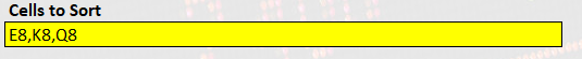
To the right of the dates, there’s another area where you can enter which cells to sort:
Cells E8, K8, and Q8 on this template are where my ‘RETURN’ headers are located, and where the percentages are. If you add sections or modify this template, you’ll need to update the cells to sort. When you update the start or end dates, the template won’t automatically re-sort until you click on this button:
If you get an error on the re-sort button, make sure you check which cells are in the Cells to Sort area and ensure that they’re correct.
#CONNECT! errors
One thing you may run into on this template are #CONNECT errors. I’ve noticed this happens once you start adding too many ticker symbols. Sometimes it’s hit or miss and you’ll get all the prices updated, but if you’re planning to list every ticker out there, just be forewarned that you might run into issues here. It’s a separate error from the #VALUE! error and one that can’t be fixed through the template, without removing some ticker symbols, anyway.
If you liked this post on the StockHistory Template, please give this site a like on Facebook and also be sure to check out some of the many templates that we have available for download. You can also follow us on Twitter and YouTube.
The Time Spent Calculator is a way to see how much time a daily, weekly, or monthly activity uses up over a long period of time.
To begin, start by using the slider to determine the number of hours or minutes the specific activity takes. Then, select Minutes or Hours from the first drop-down selection. And then below the slider, use the other drop-down option to say how often the activity happens — every day, every week, or every month.
Whenever you update one of the drop-down boxes or move the slider, the calculator will update and tell you the amount of time that you’ll spend doing that activity over the course of the month, year, decade, and 50 years.
Sensitivity analysis is a powerful way to make your template or Excel model update to reflect changes in variables. It makes it easy to run various what-if scenarios at once. In this post, I’ll show you how you can conduct sensitivity analysis in Excel in a way that’s user friendly and that can make your spreadsheet that much more versatile.
In this example, I’m going to compare two dividend stocks. One that pays a high yield right now versus one that pays a lower yield but that grows its payments over the years. I’ll look at how long it’ll take for the growing dividend to become larger than the one that’s higher today. I’ll also look at what the projections are when I make changes to my assumptions.
Setting up the analysis
First thing’s first, let’s start with the basic analysis. Once that’s setup, then we can move on to adjusting the variables and setting up the visuals. To make things simple, we’ll assume that the investment in both stocks is going to be a nice, round, $10,000.
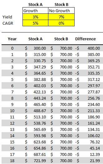
Let’s say that in our example, Stock A pays a dividend yield of 3% per year and on average it will increase its payouts by 5% ever year. Stock B, however, won’t increase its dividend payments but it currently yields 7%.
Here’s how much dividend income each stock would generate annually over the years:
Under these assumptions, it would take 18 years before Stock A begins producing more in annual dividend income.
All that this spreadsheet is doing is just taking the total investment of $10,000 and multiplying it by the dividend yield for the first year. And for subsequent years, it’s adding on the compounded annual growth rate (CAGR). That will determine what the dividend payment will be after factoring in any increase. With Stock B, since there aren’t any increases, the dividend income remains the same. Stock A, however, increases by 5% every year.
To prove the calculations out: 1.05^18 * $300 = $721.99.
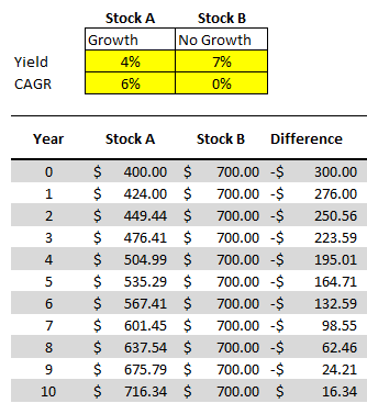
Now, suppose we change these assumptions and say that Stock A’s yield is 4% and that it grows by 6%, and Stock B’s yield remains the same. With those assumptions, it would take just 10 years before Stock A’s yield becomes the larger payout:
But rather than updating our model each and every time, we may want to have a quick glimpse as to what these differences will look like at different dividend yields.
Adding in the comparables
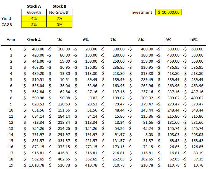
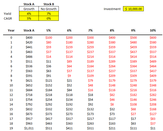
Instead of repeating these steps over and over for different stocks, to do a sensitivity analysis, I can quickly compare Stock A against a series of other stocks. For instance, I’m going to keep the assumptions for Stock A the same, and now I’ll simultaneously compare it to stocks that yield 5% all the way to 10%. I’m going to create a column for each percentage and then calculate the difference between that column and Stock A. Here’s how that looks:
All that I’m doing for these different columns is taking the value from Stock A and subtracting from it the dividend income earned at a 5% yield, at a 6% yield, 7% yield, and so on. The difference between a 4% yield and a 5% yield on $10,000 is just $100 (this the first value under the 5% column). But as the dividend rates rise, that delta grows. At a 10% yield, there’s a difference of six percentage points. That means the non-growing dividend stock pays $600 more in year 0.
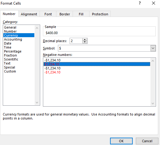
One thing that helps a sensitivity analysis chart is some formatting. First, I’ll change the format of these numbers so that negatives show up in red. I can select the cells in the other columns and change their formatting to Currency and select the red option for negative numbers:
I also removed the decimals to save space. Now, it becomes easier to see my data and when the numbers flip from positive to negative:
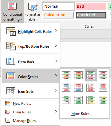
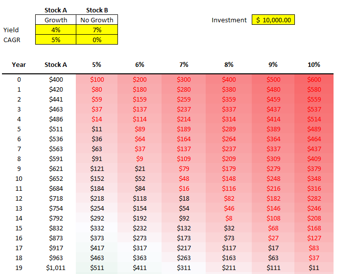
Another thing I can do is add conditional formatting. Color scales can be really helpful here, such as these ones:
Now it’s even easier to see the progression and how it relates from one dividend yield to the next:
You can adjust the formatting to how you prefer. These are just some of the ways you can help your numbers pop out.
Changing your data becomes much easier
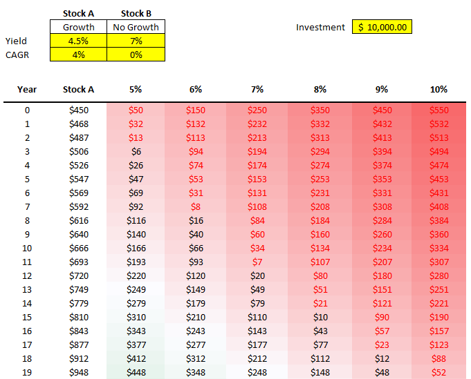
Now, what if the stock you’re comparing changes? You’ve found one that pays 4.5% and grows by 4%. You can easily change Stock A and now the rest of the values and the formatting will update:
By being able to easily update your base stock (Stock A) and then just see the changes update for all your other comparables, you can easily run through various what-if scenarios on the fly without having to update all your other formulas. That’s where a sensitivity analysis becomes very useful; it prevents you from having to repeat steps over and over to compare different scenarios. It does it all at once for you and avoids the inevitable follow-up questions you may receive in your analysis of what about this scenario or that one.
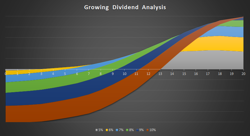
And Another way to visualize the data, is of course, through charts. And rather than a boring line chart, one that I found particularly effective to demonstrate these differences is the 100% Stacked Area Chart. Here’s how it looks like:
I only mapped the first 20 years. That’ because by that rate, it’ll capture the year when Stock A surpasses the 10% dividend yield. The chart does a great job of showing the size of the differences over the years and just how much longer it’ll take for Stock A to overtake a 5% yield versus a stock that’s yielding 10%. It’s certainly not the only chart that might work. However, it definitely has a nice effect that helps it stand out and summarizes the data well.
If you’d like to follow along, you can download the spreadsheet I created for this example here.
If you liked this post on how to do a sensitivity analysis in Excel, please give this site a like on Facebook and also be sure to check out some of the many templates that we have available for download. You can also follow us on Twitter and YouTube.
When doing any kind of data analysis, it’s important to be able to pull in not just raw data but also to show percentages. From a period-over-period percent change to how much an item represents of a total, showing a percentage can give readers multiple different viewpoints. Below, I’ll show you how to calculate percentages in Excel and to give your data more context.
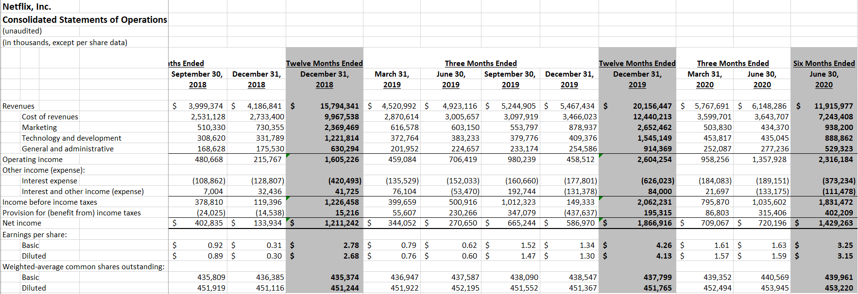
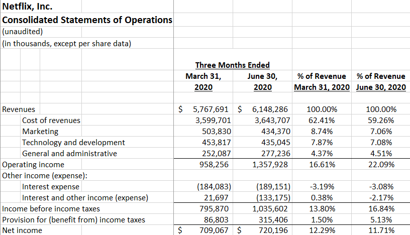
In this example, I’m going to use data from Netflix’s most recent quarterly results. The streaming giant always releases its numbers in a friendly Excel format, making it easy to analyze the data. Here’s what its income statement tab looks like, unchanged for the second quarter of fiscal 2020, which includes previous periods:
Showing period-over-period changes
Netflix’s numbers look impressive — $6.1 billion in revenue for the quarter ending June 30, 2020. However, that number on its own may not be very helpful. One way to add some context is to calculate the percentage change to show the increase or decrease from a previous period, aka its rate of growth.
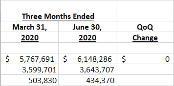
I’ll add a column next to those quarterly results and add a formula that shows the percentage difference from the previous quarter (ending March 31, 2020). To calculate the percent change, all I need is to take the difference and divide it by the old number, or base amount. A good way to remember this is: (new-old)/old.
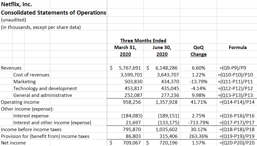
In this example, column Q contains the quarterly results for June 30 and column P is the previous period. And the revenue is in row nine. The formula for the first item looks as follows:
=(Q9-P9)/P9
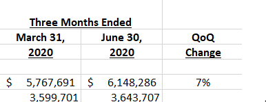
Where Q9 is the new total, while P9 is the old number. This gives me the following:
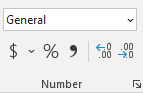
The $0 isn’t really helpful here, and it’s also not a dollar amount. Excel’s just defaulted it to that format based on the other numbers. To properly show it as a percent change, I need to change it to a % format. It’s as simple as selecting the entire column and clicking on the % sign on the Number tab:
That will now give me the following results, after centering the column:
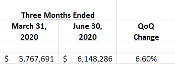
However, this still may not be ideal. If I want a bit more detail, such as to show multiple decimal places, you’ll again want to go back to the format section and select the item to add decimal places:
Clicking on this button twice will now give me a couple more decimal places:
Now, with my percentage change looking correct, I can copy the formula down for the rest of the items:
Showing the percentage of a base amount, or grand total
Another way you may want to show a percentage is how much an item makes up of a total. One common way to analyze financial statement is to look at items as a percentage of revenue. A company’s profit margin, for instance, takes its total profit and divides it by revenue to determine what percentage of its top line makes it through to the bottom line.
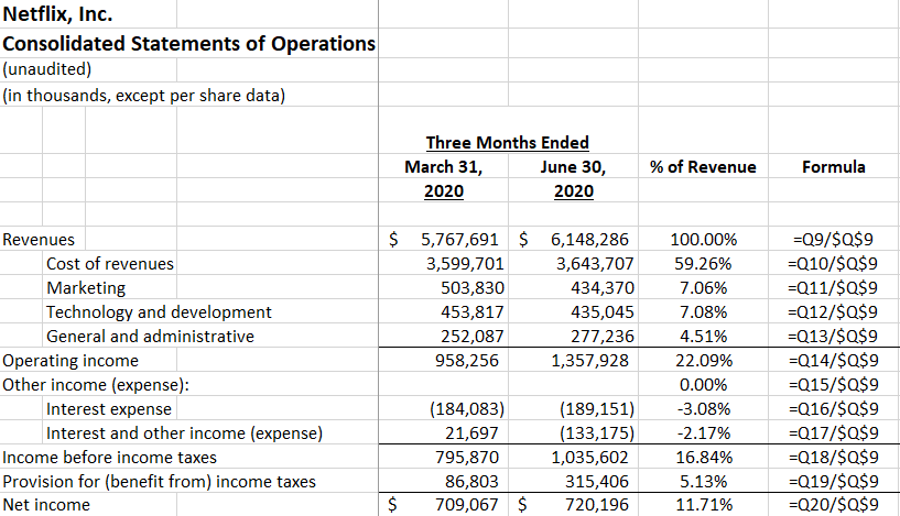
How to calculate percentages in Excel when just looking at how much an item makes up of a grand total is an easier process. In this example, the calculation just takes the current item and divides it by revenue. The key is just freezing the denominator, which in this case is revenue. Here’s how the formula looks like:
Using the % of revenue analysis, it’s easy to see that operating income was 22% of revenue and Netflix’s profit margin was 11.7%. Replicating these formulas for other periods can help compare multiple periods to see the % of revenue trends. Here’s how the current quarter looks against the previous one when looking at the percent of revenue:
Compared to the earlier quarter, Q1, the profit margin becomes a bit less impressive in Q2 as it’s declined from the previous period. Despite a stronger overall Q2 performance, a higher tax bill led to a smaller overall profit margin than in Q1.
As you can see, by adding percentages to your analysis you can create very different viewpoints and add a lot more context to the numbers.
If you liked this post on how to calculate percentages in Excel, please give this site a like on Facebook and also be sure to check out some of the many templates that we have available for download. You can also follow us on Twitter and YouTube.
VLOOKUP is a powerful function for extracting data from another sheet. And while most users will use it simply for pulling just one field, it can do a lot more than just that. Below, I’ll show you how you can extract multiple columns from just a single vlookup formula, potentially saving you from having to repeat the same formula over and over when you need more than one field.
Let’s start with the basics
First, I’ll setup a regular vlookup formula and then show you how, with a simple adjustment, you can pull a lot more data into your spreadsheet.
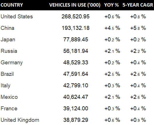
For this example, I’m going to use data from NationMaster, showing the number of vehicles in use by country. In addition to raw numbers, the data set also shows the year-over-year growth and the five-year compounded annual growth rate (CAGR). Here’s what the data looks like in my Excel sheet:
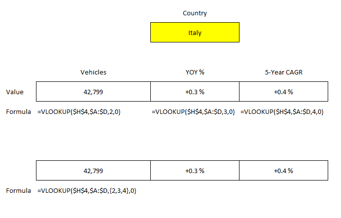
In a normal vlookup formula, you might have something like this setup if you wanted to extract all of the fields:
Cell H4 is where I’ve entered the country name. The vlookup works just fine if you want to pull data from the vehicles column. And if you want to grab the other fields you can just repeat the formula for the YOY% and 5-Year CAGR fields and just change the column number. However, there’s a much easier way to extract all those fields using just one formula.
Modifying the VLOOKUP formula
All I need to do to make this formula accommodate multiple columns is to change the column number. Rather than this:
=VLOOKUP($H$4,$A:$D,2,0)
I’ll enter in this:
=VLOOKUP($H$4,$A:$D,{2,3,4},0)
Using the curly braces, you can specify the different column numbers that you want to extract. Since this is an array formula, on older versions of Excel you may need to enter ALT+SHIFT+ENTER for the calculation to work properly.
Here’s the difference in formulas:
The columns you want to extract also don’t need to be sequential. You can extract columns 2 and 4 rather than all three. All you need to do is separate the column numbers that you want with a comma.
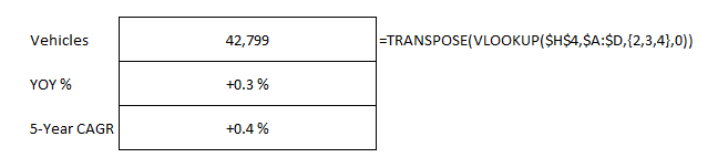
Retrieving the fields vertically instead of horizontally
Depending on how you’ve got your sheet set up, you may prefer for the data to come back in rows rather than columns. This too, is an easy fix.
All that you need to do is wrap your existing formula within the TRANSPOSE function. Here’s what the updated formula looks like:
=TRANSPOSE(VLOOKUP($H$4,$A:$D,{2,3,4},0))
This again is an array formula so you may need to use CTRL+SHIFT+ENTER on older versions of Excel. But doing it will allow you to retrieve the values vertically:
There’s a lot of flexibility with how you can use vlookup to extract data that can allow you to not only simplify your spreadsheet but also result in having to create fewer formulas.
If you liked this post on how to extract multiple columns from vlookup, please give this site a like on Facebook and also be sure to check out some of the many templates that we have available for download. You can also follow us on Twitter and YouTube.
For a while, one of the big advantages Google Sheets had over Excel was the ability to pull stock quotes easily. But that’s no longer the case as there is a new function in Excel that allows you to pull in stock price history. Below, I’ll cover how to use the StockHistory function.
How the function works
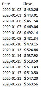
The function itself is fairly simple and requires just two arguments at a minimum, and that’s the stock ticker and the start date. By default, the function will return the closing prices from the start date until today. For instance, if I want to pull Tesla’s share price since the start of the year, this is what my formula will look like:
=STOCKHISTORY(“TSLA”,”2020-01-01″)
The formula will then generate an array. Here’s a portion of what it looks like:
If you want to pull just the most recent share price, here’s what you can do:
=STOCKHISTORY(“TSLA”,WORKDAY(TODAY(),-1))
Using the WORKDAY formula you can ensure that you’re going back one business day. You may need to adjust this if you’re on a weekend but basically you just need to manipulate the date to make this work. Note that this doesn’t appear to give you the current day’s close. When I ran this on a Friday, the most recent closing price it returned was from Thursday’s close. It’s clear this function’s intended for historical data rather than live or even delayed stock prices.
If you want to specify an end date for your data, you can enter a date in the third argument, right after the start date.
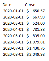
The function gives you many options, including which data points you want to pull in and what intervals you want. You can pull prices on a monthly or weekly basis by selecting either a 0 (daily), 1 (weekly), or 2 (monthly) for the interval argument. Here’s how I’d pull monthly prices for Tesla:
=STOCKHISTORY(“TSLA”,”2020-01-01″,,2)
It’s important to note that these aren’t monthly averages, they’re just the stock prices as of the end of the specified month. Although the date for the first entry suggests January 1 (the markets weren’t open that day), that’s actually the January 31 closing price.
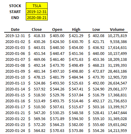
You can choose whether you want to see the headers and you can also add more fields, including the opening price, the high, the low, and the volume. You can even determine if you want to even see the date (although that’s probably not a good idea when you’re looking at historical data).
It’s easy to make a template with this function since it populates the data for you. Using variables for the ticker, the start date, and the end date, I can quickly set up a sheet that’s easily updatable:
The only formula that I enter is the one cell for the STOCKHISTORY function:
=STOCKHISTORY(C2,C3,C4,0,1,0,1,2,3,4,5)
Where C2, C3, and C4 refer to the stock, start, and end dates. The numbers 1 through 5 are needed to ensure that all the fields are extracted.
If you want more details about this function including the different arguments, you can check out Microsoft’s official page for this function.
How can I get other (non-US) tickers?
One of the things you’ll notice from the above examples is that I didn’t enter any prefix for the stock ticker. The StockHistory function knew I was looking for Tesla’s stock price. However, if you want to pull data from other exchanges, including those outside the U.S. markets, you’ll need to add a prefix to make sure that you’re getting the right quote. And since the function won’t actually return the company name, you need to make sure you’re entering the ticker correctly into the function.
Refer to this link for all the different market identifiers. For instance, if I wanted to pull the share price of Air Canada, which trades on the Toronto Stock Exchange, I’d need to enter the ticker as follows:
XTSE:AC
In most cases, it looks as though it’s just an X before the exchange’s usual prefix but you’ll want to double check to make sure.
Why you may not find the StockHistory function on your version of Excel
Since the function’s in beta, StockHistory is not available for most users. You can, however, sign up for Microsoft’s Office Insider program which will give you access to functions while they’re in beta. To join the program, follow the steps outlined here.
If you liked this post on How to Use the New Stock History Function in Excel, please give this site a like on Facebook and also be sure to check out some of the many templates that we have available for download. You can also follow us on Twitter and YouTube.