Merged cells are great for presentation purposes but not so ideal when you’re creating a model or a complex spreadsheet. It can make copying cells or formulas painful as you can get an error or unintended results when doing so. However, there’s a way that you can achieve the same result as a merged cell without actually having to merge anything.
Align cells rather than merge them
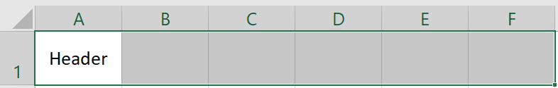
When merging cells, you would select the cells you want to merge, and then click on the following button:
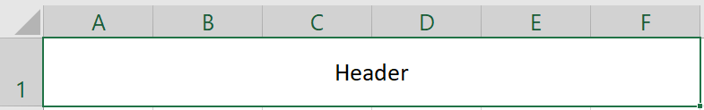
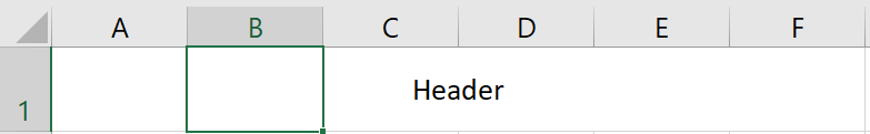
What happens in that case is that the cells you selected now become one. In the below example, if I click on Merge & Center, the text would get spread across multiple cells:
And become this:
By doing so, I can no longer enter a value individually in cells B1:F1 as the merged cell effectively takes over. If you never plan to copy over these cells then that’s fine but if you do, then you could end up with some annoying errors along the way.
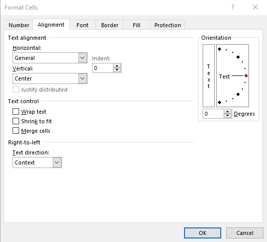
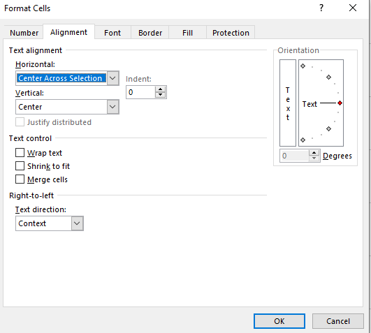
However, there’s an easier, less intrusive way of accomplishing the same result. I would still select cells A1:F1 but instead of using the Merge & Center button I’ll go into the cell formatting menu (CTRL+1) which will give me the following options:
From here, I’ll adjust the Horizontal Alignment and select Center Across Selection:
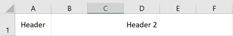
Now, my text is spread across those cells but it isn’t merged, it only looks that way. For example, I can still click individually on cell B1 and enter data there:
And if I do that, it takes over the center alignment and pushes back the other text into cell A1:
The advantage of using an alignment rather than merging cell is this avoids the errors that can come when you’re modifying or copying data and you get notifications that the cells are not the same size.
By using the horizontal alignment, you have the flexibility of making your text appear as if you’ve merged it across multiple cells without you needing to unmerge data later on if you want to change the text or add data.
If you liked this post on an alternative to merged cells please give this site a like on Facebook and also be sure to check out some of the many templates that we have available for download. You can also follow us on Twitter.
When you’re dealing with complex spreadsheets in Excel, it can sometimes be difficult to tell which cells are safe to delete and which ones you need to keep to ensure everything is working properly. Even cells that look empty could contain formulas. And deleting them can cause problems and wreak your spreadsheet. Before you delete a formula, there’s one thing you can do to prevent that mistake:
Check for dependent cells
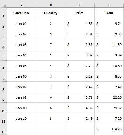
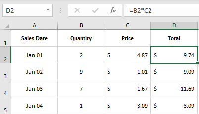
If you’re not sure if a cell is okay to delete and if it has any other cells that depend on it, you can check for dependents. Before deleting a cell, you can click on CTRL + ] which will highlight any cells that use the active cell in a formula (on the current sheet). Here’s a sample spreadsheet that lists price, quantity, and multiples them to get to a total price:
The formula in column D multiples the value in B by C. So that means the value in D depends on the values in C and B (the exception is the subtotal, which depends on the values above it). If I select cell C2 and click on CTRL+], it takes me to cell D2:
If there is more than one cell that depends on the active cell, then Excel will highlight all of them.
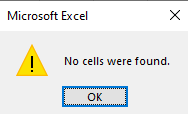
What if there aren’t any dependent cells? In that case, you’ll get the following message:
If you get this message, that means you’re safe to delete the current cell as nothing in the current sheet links to it. However, the one limitation of using the shortcut is that it may not be easy to see all the cells that depend on that one cell. It also won’t tell you if there is a cell on another sheet that uses it.
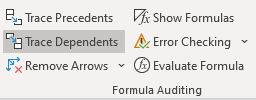
What you can do is use the Trace Dependents button in Excel, which is on the Formulas tab:
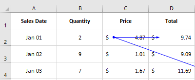
By clicking on this button, arrows will now show up telling me exactly where the dependent cells are:
In this situation, the arrow clearly shows an arrow pointing to cell D2. Let’s say I also use the cell in a formula in some place far off in a the same sheet:
Another line will point to the other cell. If you have a large data model that goes on for many rows and columns, it may not be obvious where the dependent cells are if you use the shortcut key. Using the shortcut can be helpful as a quick check but if you actually want to see all the cells that use the active cell, you’re better off clicking the Trace Dependents button.
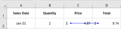
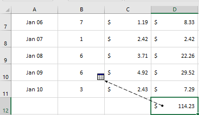
Next, let’s go to the subtotal. Here, let’s assume I’m using this total somewhere on another sheet. Using CTRL+] won’t help me much in this case as it will tell me no cells were found (assuming no cells on the current sheet link to it). But if I click on Trace Dependents, it will show that there is a dependent cell on another sheet:
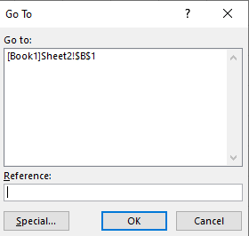
If you double-click on the dotted line (the portion that’s within the cell), the following box will pop up:
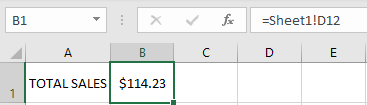
This tells us that there is a dependent cell on Sheet2, cell B1. I can go there manually or I can click on the selection and then press OK. Then it will take me directly to the cell:
This isn’t practical on a wide scale as you would have to go one by one and you could have arrows going all over the place. But if you’re not sure about a certain cell, using the Trace Dependents button can be a quick way to see if it’s safe to delete the cell.
If you liked this post on 1 mistake to avoid when deleting formulas in Excel please give this site a like on Facebook and also be sure to check out some of the many templates that we have available for download. You can also follow us on Twitter and YouTube.
You can use Excel to create models, templates, and also to do analysis. This will be the first in a new series of posts to do with Excel-related analysis and how to set up a question and answer it accurately. In this analysis, I’m going to look at how much money you can be losing by letting it sit idle. Specifically, I’ll analyze an investment that pays you a dividend every quarter and look at two scenarios — one where you reinvest dividends back into the stock and one where you don’t. How much of a difference that can make over a 30-year period could surprise you.
At the bottom of the page, I’ll leave the file available for download if you want to take a look at my work and follow along and to see just how much of a difference there is when you don’t reinvest dividends.
Scenario 1: collecting the dividend payments and not reinvesting them
The assumptions and fields
In the simplest scenario, let’s set it up that you don’t reinvest dividends back into the company. To create a template for this in Excel, we’ll need to know the price of the stock, how much you’re investing, and how much the company pays in dividends (which is usually on a quarterly basis), and the growth rate. To keep it simple, we’ll assume the dividend payments will never change and so the amount that you receive in dividends will remain constant.
This is a useful assumption to make when making this type of comparison so that you can isolate one variable, which in this case is whether you reinvest the dividend payments or not. It’s safe to assume if there is a benefit of reinvesting dividend payments, it’ll be even greater if the payouts increase over time, so it’s unnecessary to incorporate dividend growth into the model in order to do this analysis.
I’ll also set the price of the stock at $100, the quarterly dividend at $1.25, and the amount to invest at $10,000. There will be a calculated field to determine the number of shares, which will take the amount invested and divide that by the price of the stock. With a $10,000 investment, you would be able to own 100 shares of a stock that’s priced at $100. I’ll also assume that the stock will rise by 5% every year. These are what my inputs and calculations look like so far:
Setting up the headers
Next, we’ll need to set up the headers for the actual model where the results will be populated. The fields I’ll include are the year, the starting portfolio value, the dividend amount, the cumulative dividend, the ending portfolio value, and the portfolio + dividend.
In the year field, I’m just going to increment the numbers 1 to 30 to show the portfolio’s progression over 30 years. You can do this a few different ways. Besides manually entering the numbers 1 to 30 in, you can enter the number 1 in first and then create a formula that just adds one to the number above, and then copy it down. Another option is to enter the values 1 and 2 in the first two rows, select those two cells, and then copy that down. Since you are selecting multiple items, Excel will know the pattern and that you want to increment by 1 each time. Otherwise, just trying to copy 1 down will give you a series of 1’s. For some examples of how this works, check out this post on how to autofill data in Excel.
For the starting portfolio value, I will just link to the initial amount invested and in subsequent periods this will be equal to the previous year’s ending portfolio value.
To calculate the dividend amount, all I need to do here is enter the number of shares, multiply them by the quarterly dividend, and then multiply that by 4, since the payments are quarterly. My formula looks as follows in the first cell:
=$C$7*$C$3*4
$C$7 is the number of shares and $C$3 is the quarterly dividend. Since I’m not reinvesting any dividends, my amount invested will remain the same and that also means that I won’t collect more dividends (since I’m assuming the dividend rate will remain unchanged). This means that every year, I’m expecting to collect $500 in dividend income as I’m taking 100 shares, multiplying them by $1.25 and then by 4 payments.
The cumulative dividend field is an easy calculation as it’s just adding the total of all the dividend payments. You can calculate the cumulative value by using the SUM formula, freezing the first cell, but not the last one. In cell D12, my formula looks as follows:
=SUM($C$12:C12)
My dividend payments are in column C. While the first cell is frozen, the second one is not and the calculation will expand as I copy this formula down.
The ending portfolio value is calculated by taking the starting portfolio value and multiplying it by the growth factor — which in this case is 5%.
The last formula is the portfolio + dividend calculation. This will tell me what the total value of my investment is after factoring the growth in share price as well as all the dividend income I’ve collected over the years. This is a simple calculation of just adding the ending portfolio value (in column E) with the cumulative dividend in column D).
With all of my formulas copied down, this is what my values look like over the 30-year period:
The dividend payments total $15,000 after 30 years and the portfolio will rise to a value of $43,219.42 by the end of the period. Combined, the value of this investment is $58,219.42 when adding the dividend income on top of all the growth the stock is expected to achieve over the years.
Now, let’s switch over to the other scenario, where you reinvest dividends to buy more shares of the company.
Scenario 2: reinvesting the dividend income
This scenario will be more complicated because now the number of shares owned will change every year if you were to reinvest the full amount of dividends you earn.
I’ll need to make some changes to the structure of the template. First, I’ll want to track the number of shares that are owned over the years as that will determine how much dividends will be collected. I’ll also need to calculate the expected stock price to determine how many additional shares I can buy with the dividend income. And I also won’t need the cumulative dividend since the payments will be reinvested back into the stock.
The stock price field will rise by 5% each year and its formula will be simple as it will just rise by the growth rate. As for the number of shares, that will start with the initial purchase of 100 shares and then in future periods it will take the dividend amount and divide it by the stock price to determine the number of additional shares that can be purchased. The dividend calculation will then take the number of shares, multiply it by the quarterly dividend and then again by 4 quarters
With those changes, here’s what the model looks like if the dividend income is reinvested:
At $92,169.05, you’re making $33,949.62 more by reinvesting the dividend back into the stock. This, of course, assumes that the stock will continue to grow at a rate of 5% and that you’ll do nothing with that dividend income but let it sit in the first scenario. But the point is still the same: the cost of letting money sit idle can be significant. In the second scenario, your portfolio will be worth 58% more than it would be in the first scenario.
Now, if you were to invest the dividend income from the first scenario into other investments, then the difference would likely be smaller. However, for the purpose of this analysis, it’s clear that there’s a big advantage of reinvesting dividend income. One variable that wasn’t considered in this analysis is the discount that companies sometimes offer investors when reinvesting dividend income, which could result in more shares and greater returns over the long term under the second scenario. But again, for the sake of simplicity, that was left out but it’s an example of another reason why reinvesting dividend income can be very beneficial.
Proving out the variances
The last part of this analysis involves proving these differences out, comparing when you reinvest dividends versus when you don’t. This is an important part in order to show where the variances came from and to illustrate that the calculations are correct.
Two key areas that contribute to the differences between these two models are the loss of dividend income by not holding more shares and also the loss of portfolio value by not benefiting from the full incremental growth each year.
To do this, let’s create another table that summarizes the variances. The first field here will be the portfolio change, which will just look at the difference in portfolio values between the two models in each year.
Next, the loss of growth column will calculate how much growth is lost by not reinvesting the dividend income. This is calculated by taking the difference in starting values and multiplying that by the growth factor of 5%. Since the dividend income isn’t reinvested, the starting portfolio value will be lower in the first scenario, which means the amount of growth earned will be less than under the second scenario.
The loss of dividend income is the next source of variation because with fewer shares in the first scenario, that will mean less dividend income. To calculate this variance, we’ll need to take the difference in the number of shares and multiply that by the quarterly dividend and by 4, for the number of payments during the year.
Lastly, there is a field for the cumulative loss, which is important as it’s a running total of the losses from dividend income and growth. This should match up the total portfolio change field, and I’ve added a check column to calculate the difference and ensure everything nets out to zero.
Here’s what the variance table looks like:
As you can see, the bulk of the losses originate from the loss of growth as the impact of compounding can significantly affect your overall returns over the long term when you don’t reinvest dividends.
To see this file in more detail, you can download it from here.
If you liked this post on whether you should reinvest dividends or not, please give this site a like on Facebook and also be sure to check out some of the many templates that we have available for download. You can also follow us on Twitter and YouTube.
Are you looking for an easy way to log and track your time in Excel? Below, I’ll show you how you can keep track of the time you spend on tasks without the need for a complicated template or to even open up Excel every time to enter in your time. With a combination of Excel and Notepad, you have all the tools you need to quickly and easily track your time and create a log in Excel.
An easy trick to turn Notepad into a log
To make the process of logging time easy, you probably don’t want to have to open up an Excel spreadsheet each time. There’s an easier way to do so and that’s by using Notepad. Open up a new instance of Notepad and write the following in the first line:
.LOG
Save the file as whatever you want, and then close it. Open it up again and you’ll notice there is now a timestamp when you open the file. Because you entered .LOG at the start of the Notepad file, it will now automatically create a timestamp each and every time that you open the file.
Now, when you’re working on a task, just enter in some text, such as “working on Excel,” click save, and close the file. Now, when you’re switching over to another task or want to say that you’ve finished the task, open up the text file again and enter in a new entry. You probably don’t need to say that you’ve ended a task since the start of a new task would effectively tell you that the previous one is over.
The key thing to remember when you’re logging your tasks in Notepad is that you’ll want to save the file once you’ve made an entry, and then close it out. A good place to store the file might be online or on a shared folder, somewhere that you can access it from any computer and that you can easily update from wherever you are. As you keep adding to the log, you’re essentially creating a database of all your entries.
You can create multiple log files depending on what you’re tracking or you can just keep one big list in a single text file. Either way, once you’ve made some entries, what you can do is now extract that time log in Excel, which brings us to the next step:
Pulling the data into Excel
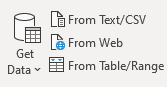
The text file, while useful, isn’t going to be terribly helpful if you want to easily see the time you’ve spent on a given task. This is where Excel can be incredibly useful. To get the information into Excel, go onto the Data tab and import data using the From Text/CSV button.
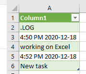
You can leave the default settings and Load the data as is as it’ll likely leave all your text entries in vertical form, which will still work for our purposes. Here’s a sample of what my log file looks like after importing it into Excel:
If you’re using one of the newer versions of Excel that includes PowerQuery, a connection is created when you import the text file into your spreadsheet. This prevents you from having to re-import the file manually each time to check for changes. You only need to refresh the data and it will pull in the changes for you.
And if you make additional entries to your text file, save it, and refresh the data in the spreadsheet and it will update. Just simply right-click on one of the entries in column A, select Refresh, and the data will update from the file — as long as it remains saved in the same place.
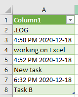
If, after an hour I make another entry to make log file and click on update in the Excel file, the information is up-to-date without having to initiate another import process:
This is where Excel is very powerful and effective in making it easy to pull data from another file. However, the data isn’t in a form that’s terribly useful to us in the form that it’s in now. Let’s move on to the next part: setting up the template in Excel so that the time log will be a lot more user friendly.
Creating a template to populate the information correctly
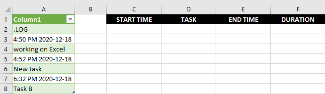
The data is in column A, and what I’ll do is create headers in columns C:F for the Start Time, the Task itself, the End Time, and the Duration (in minutes). Here’s what that looks like:
Now, I’ll need to enter in formulas to populate all those fields. The start time field will initially pull from the third row in column A, and then it will grab every second row after that. So let’s start with building out that logic.
I’ll start with using an INDEX() formula to pull a value from column A. Since there’s only one column I’ll be extracting data from, the key argument is going to be the row number. The third row is where my first entry is, so for the row number I’ll start with the number three. Here’s what my formula looks like thus far:
=INDEX(A:A,3,1)
I select row 3 and column 1. This will only work for the first value. I need to adjust the formula so that it will automatically adjust based on which row I’m on, so that it knows to take either the first time entry, the second, the third, and so on. The ROW() function is helpful in this case because it will return the row number of the current cell. And since my first entry in the table will be on the second row, I’ll want to remove the first two rows. My row calculation looks like this right now:
3+ROW(C2)-2
For the first entry (on the second row), this will evaluate out to 3, since ROW(C2) will equal 2 and it will minus 2 from that. This still works for the first entry, but if I were to copy this formula down it would not give me the correct result for other entries. For instance, in row 3, the formula would be as follows:
3+ROW(C3)-2 this would evaluate to 3+(3)-2 = 4
But row 4 contains my task description, not the next timestamp. I need to double with each row I go down. I need to adjust my formula for the row calculation back in C2 to be as follows:
3+(ROW(C2)-2)*2
Now, the row number minus 2 will then multiply by 2. If I copy this formula down to cell C3, it’ll look as follows:
3+(ROW(C3)-2)*2 : this would evaluate to 3+(3-2)*2 = 3+(1)*2 = 5
This returns row 5, which is the next timestamp in column A. If I copy the formula down to row 4, then it will return the 7th item in the column, which is again the next timestamp. Now that the formula is correctly returning each odd-numbered row, I can use this formula for the template I’ve created. My full formula in column C2 looks as follows:
=INDEX(A:A,3+(ROW(C2)-2)*2,1)
This will work not only for the initial timestamp but it will also extract entries that come after it. All you need to do is copy the formula down.
I can replicate this for the Task field in column D. The only change I need to make is to use row 4 as my starting point rather than 3. And so my formula for the task column looks as follows:
=INDEX(A:A,4+(ROW(C2)-2)*2,1)
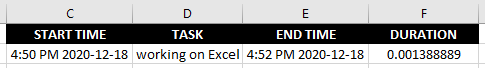
For the end time, I’ll use row 5 as my starting point. The end of one task will be the same as the start of the next task. And then all that’s left is to calculate the task duration in column F. The calculate the difference in times, I’ll start by taking the end time and subtracting the start time. However, this will give me a decimal that isn’t very easy to interpret:
The reason is that Excel converts this into a fraction of a day. A two-minute interval is less than 1% of the 1,440 minutes that are in each day, which is why the number is so low. To convert the duration into hours I can multiply it by 24, and then the number changes to 0.033, which is the fraction of an hour that two minutes represents. But if I want to go further and convert this into total minutes, I’ll multiply this again by a factor of 60. Now my formula looks as follows:
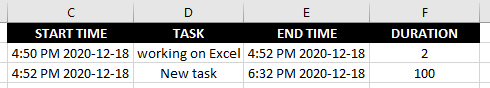
=(E2-C2)*24*60
Now, after rounding off the decimal points, my duration calculation in column F correctly gives me the number of minutes between the start and end time of a task:
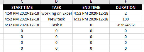
The table is now set up and you can just copy these formulas down to accommodate more entries. You’ll end up with a series of zeroes if there’s not enough data in column A. If you want a cleaner solution, what you can do is use the COUNTA() function to determine the number of rows that are in column A and determine whether to apply a formula or not. For instance, in my example, my data goes until the 8th row and so my formulas look fine for the first two entries but after that, there is no end time for the third task and the subsequent entries are full of zeroes:
It’s not a terribly elegant solution at this point. To get around this, I’ll create a rule for each column to say that if there is no entry, it will be blank. For the start time, I’ll add the following to the beginning of the formula:
IF(COUNTA(A:A)<(3+(ROW(C2)-2)*2),””
This will check if there are enough rows in column A to extract a value for the current cell. If not, the value will be blank. Here’s how the full formula looks in cell C2:
For the duration calculation, I will check to make sure there are values in both the start and end time, otherwise, the value will be blank:
=IF(OR(C2=””,E2=””),””,(E2-C2)*24*60)
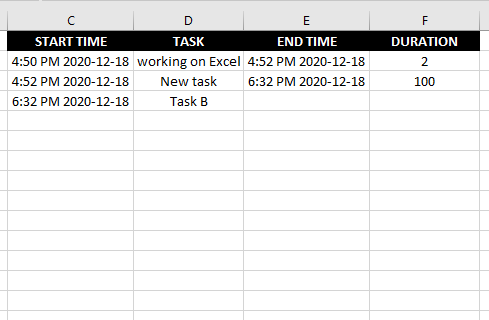
With these formulas now set up, I can copy them down hundreds of rows down if I want and they won’t result in a series of zeroes or errors:
The data in Excel will now auto-populate as I add more entries to the time log and at the same time it won’t be an eyesore if there is incomplete data.
If you liked this post on how to create a time log in Excel, please give this site a like on Facebook and also be sure to check out some of the many templates that we have available for download. You can also follow us on Twitter and YouTube.
To enter data in the price to earnings ratio calculator, start from top to bottom. Tabbing over or hitting enter will update the calculations.
Current Stock Information
Price $
EPS $
P/E
What-if Analysis
Change
to
What P/E is and why it’s important for investors
The price-to-earnings (P/E) ratio is a key metric that many investors use when analyzing whether a stock is well-priced and a good buy, given its level of earnings. The calculation takes the current stock price and divides it by the company’s earnings per share, typically over the last four quarters. You can also calculate a forwardP/E. This is what the ratio will be in the future, based on estimates of earnings.
This is a particularly useful calculation in a year like 2020 when the coronavirus pandemic has thrown many businesses out of whack and some are over or underperforming. And that means their P/E ratios may not be all that reliable right now.
Using a P/E ratio is particularly useful when comparing one stock against another. If a stock is trading at a very high P/E of 50 or more, it could be a sign that it’s overvalued. However, this can be skewed if a company is coming off a bad quarter where its profits were low. It’s always important to consider the context. And comparing different types of industries may not be helpful, either. A bank stock that is relatively stable and that may not achieve much growth will trade at a much lower P/E than a high-growth tech stock where its sales are climbing by 50% or more.
How to use this calculator
I wanted to create a calculator that could be useful for setting up alerts. For instance, if a stock is trading at a P/E of 50 and you want to set up an alert for when it falls to a lower multiple. You can use the What-if analysis section to plug in the P/E that you want to buy it at. It will then tell you the price it will have to fall to or the EPS that it will need to rise to.
You could also use it as a simple P/E calculator. While many financial websites may give you a P/E number they won’t always update quickly, like when a company reports its earnings. If you know what the new P/E is, you can plug it into the calculator. You can also do a what-if analysis to see what the ratio will be if earnings rises or falls to a certain number.
To enter data into this calculator, you’ll want to start from the top and work your way down. Enter the price and EPS first and then make your selections in the what-if analysis. If you go straight to the what-if analysis then the calculation won’t be correct. As you’re entering data and tabbing over, the formulas will automatically update. Hitting enter after entering in a number will also update the calculation.
Another calculator you may want to try is the average down calculator, which can help you determine how many more shares you’ll need to buy to get your average price down to a specified amount.
If you liked this post on the price to earnings ratio calculator, please give this site a like on Facebook and also be sure to check out some of the many templates that we have available for download. You can also follow us on Twitter and YouTube.
Spreadsheets can allow you to analyze data and create reports efficiently. But sometimes the tasks that are involved can be difficult or appear to be time-consuming. The good news is that there’s a lot of automation you can achieve in Excel, and it isn’t always necessary to know how to code in order to do so. Below, I’ll show you 10 types of tasks that you can automate in Excel either on your own or with our help.
1. Cleaning and parsing data
One of the more challenging things in Excel is when you’re dealing with a dataset that may not be easy to manipulate. For instance, if you’ve got text mixed in with numbers or dates that aren’t in the right format, Excel may not interpret or recognize the data properly. But there are many formulas that can help you with that. Rather than manually fixing the data, you can use functions like TRIM, CLEAN, LEFT, MID, and RIGHT to extract what you need while also getting rid of extra, unnecessary spaces and other characters.
If you’re looking for more of a walkthrough of the process, there’s a detailed explanation in this post of how to parse data.
Through the use of formulas, you can save hours that you might otherwise spend trying to clean up your spreadsheet. And the best part is that once you’ve set it up, you can re-use the formulas as you add more data. You don’t need to use macros or complicated coding to clean up; a well-structured template can be enough to do the job for you.
2. Creating simple reports
One of the best features of using Excel is that once you’ve entered data into a spreadsheet, it’s even easier to create a report from it. One example is through the use of a pivot table, where through just a few clicks you can easily summarize your data and split it along different categories. Slicers can make filtering and summarizing data even easier in pivot tables, especially for users who aren’t very familiar with Excel. Forget any manual work here; just a few clicks and you’ve got a report that can quickly summarize information in a table for you!
Alternatively, you can also insert charts easily and Excel will try and select the best one based on your data set. There’s also lots of formatting you can apply to charts so that they have the look and feel that you’re after. And once you’ve got a look that works, you can re-use it over and over again.
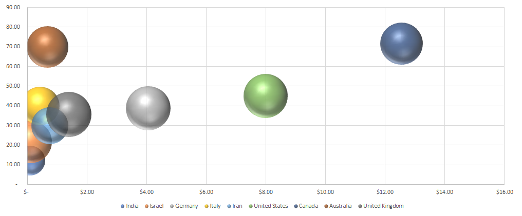
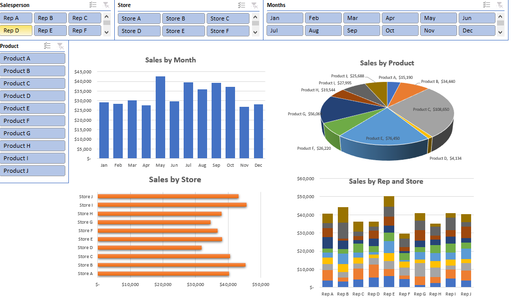
3. Creating dynamic dashboards
Dashboards are incredibly popular but they can be complex to set up. Then there’s also the challenge of updating it and making sure the data is up-to-date. It can easily take you hours every time to make sure the information is accurate.
However, in this post, I show you how to create a dynamic dashboard that not only won’t take you hours but that will automatically update as you add data to it. And then, you end up with a report that looks great to send to management to easily review and update.
4. Routine data entry
One of the biggest headaches people can face when using spreadsheets is when they hard-code calculations. A hard-coded calculation is where you don’t reference any cells and just put the result in the cell; it can make it nearly impossible to decipher how that number was calculated (especially if you’re not the person who entered the value). If you go to re-calculate it or update it, you could spend a lot of time just trying to figure out the calculation.
However, by using a formula, there’s no ambiguity as to how a value was calculated. Not only does that save you the time of entering in data but it also makes it easy to correct and update the figure. Ideally, you should minimize the number of places you’re manually entering data into. By doing that, you’ll have a much more robust template where your inputs are kept to a minimum which will eliminate the need for a lot of data entry and your other calculated fields will update automatically. This type of automation doesn’t require complex coding and just needs an Excel spreadsheet to be carefully constructed so that it is efficient and makes the most of formulas.
5. Conditional formatting
Oftentimes you’ll want to color-code your data to highlight things you should be paying attention to. If you’ve got an aged accounts receivable schedule, it is useful to highlight which accounts are more than 90 days overdue. You could manually filter the data and highlight all the cells or rows in red that are overdue, but you can just use conditional formatting to do that for you.
Through conditional formatting, you can create rules to determine when a cell or row should be highlighted in red, when you may want it to be in yellow, or when you may just want to hide the text so that you can easily skip over it. For example, hiding zero values can make it easy to focus on more important numbers.
You can apply many different formatting rules and can even put in a hierarchy to determine if you want to keep applying formatting rules or whether you want to stop if a specific criteria is met. Conditional formatting can be complex but it can be a huge time-saver by allowing you to focus on just the items that are important to you. And once you’ve set up the rules, you don’t need to worry about making changes every time you add new data.
If you use multiple workbooks, then another area where you can avoid re-entering data is by linking both workbooks. There are numerous ways that you can do this. One approach involves just linking directly to another worksheet where data will automatically pull from another table.
You can also use the INDIRECT function to reference another worksheet or workbook. Just like with a template, once you set up these formulas and connections, they are there to stay and you can avoid having to manually make changes by yourself.
7. Audit tracking by logging changes
One of the neat features of many Office products is they allow you to track changes that are made. This is normally when you share a workbook with other users. However, through the use of macros, you can have a separate sheet that can tell you which values were changed, when, and by who.
Rather than manually noting these changes or relying on people to make the updates themselves, it doesn’t take much effort through a macro to create a log of what’s been changed.
8. Generating PDFs
One thing many advanced Excel users like to do is to use automation to export reports into PDFs. While there is a way to print to PDF, and it’s particularly easy on the newer versions of Excel, it can be a time-consuming process especially when you need to print out multiple sheets. Here again, with a simple macro, you can auto-generate PDFs and save them in a predefined folder all with the click of a button.
9. Sending emails
Another feature many users like is the ability to use automation to send out emails right from Excel. Through the use of macros, this is also possible. You can create a macro that will enter in the email of the recipient, attach a file, enter the body of the message, and even send the email itself. This can be even set up on a large scale, such as sending out invoices to dozens or hundreds of customers, a process that could easily save you hours worth of work.
10. Just about anything else with VBA
The power of programming in Excel can unlock many different possibilities with what you can automate. Whether it’s using automation to help import data and then manipulating it, creating custom reports, or following a series of complicated steps, there are many tasks in Excel that can be expedited with a few clicks of a button. As long as there’s some logic to the process that you can break into steps, then you can also build that into the code and automate it.
Don’t know where to start? Contact us!
There is significant potential in Excel but not everyone knows how to use automation to make the most of it and to make a spreadsheet as efficient as it can be. You can contact us if you have a certain Excel issue that you need help with or if one of the tasks above has perked your interest and you’d like to learn more. We can help create solutions for you that work efficiently and that can save you many hours, perhaps even days every month.
If you liked this post on 10 Tasks You Can Automate Today, please give this site a like on Facebook and also be sure to check out some of the many templates that we have available for download. You can also follow us on Twitter and YouTube.
Do you want to know how to calculate how many hours and minutes have elapsed between two times? Below, I’ll show you how to do that with Excel formulas. The difference won’t be in just fractions of days or hours but real minutes and hours that make it easy to measure. To make this work, however, the first step is entering in the time correctly.
How to enter time in Excel
Excel has a built-in time function called TIME where you can enter the hour, minute, and second. For example, if you wanted to enter a time of 6:30 AM, you could enter a formula of TIME(6,30,0). Alternatively, you could type in 6:30 AM — the key is leaving the space between the time and the AM/PM indicator.
However, the one clear limitation here is that this won’t help you if you want to calculate the hours and minutes between times that span more than just one day. By using the TIME function, or entering just the hours and minutes, Excel is always going to assume you’re talking about the current day.
The best way to enter in time is to also factor in the date. Depending on your regional settings you might enter this differently, but this is how I’d enter a time of 8:00 PM on Nov. 20 on my computer:
2020-11-20 8:00 PM
I can also use a 24-hour clock and type in the following:
2020-11-20 20:00
Either way, Excel knows what time I’m talking about. If you always want to return the current time, you can use the NOW function.
For the start time, I’ll set it to the start of the year: 2020-01-01 0:00
Calculating the difference
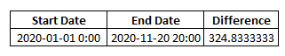
Just using the minus operator, I can get the difference between these two dates as follows:
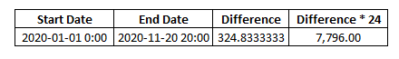
By default, Excel will return the number of days, including the fractional days as well. To convert days and calculate the hours instead, we will multiply the difference by 24, since that’s how many hours are in a day. That gives us the following:
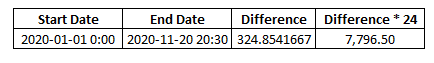
That’s 7,796 hours between those two dates and times. It’s a nice round number but what if we changed it so that the end date was at 8:30 pm, or 20:30, this is what the updated calculation would look like:
Now I’ve got that residual 0.50 which indicates half an hour. But I want minutes, not fractions of an hour. The easiest way to do this is to create one calculation for hours, and another for minutes. Then, afterwards, you can concatenate them together. To get the total hours, I’ll adjust my formula to include the ROUNDDOWN function so that it does not include the 0.5. It looks something like this:
=ROUNDDOWN(datedifference*24,0)
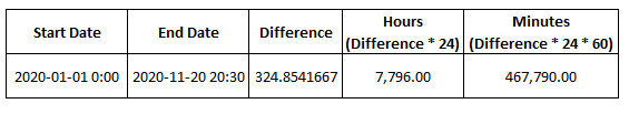
Where datedifference is that raw calculation between the two dates and times. In my calculation, I’m still multiplying the time difference by 24 to get to hours, and then I round that to 0 spots, which is indicated by the 0 in the second argument. Now it will only show 7,796.00 for hours.
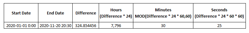
To calculate the number of minutes, I’ll need to multiply the datedifference by 24 and then again by 60, to convert the difference into minutes. This is what my calculations look like thus far:
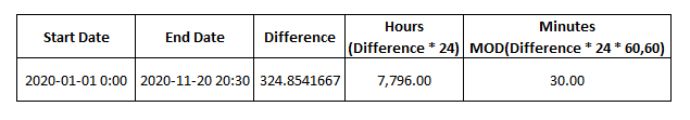
My hours are nicely rounded but my minutes include the total minutes, which is not what I want. I only want the minutes that are left over after the hours are factored out. Here I can make use of the MOD function which will tell me the remainder after division. I’ll adjust the minute calculation to calculate the remainder after I’ve divided the total minutes by 60. This will determine what’s left over after pulling out full 60-minute hours, which is that residual 0.50 that I’m after. Here’s what this formula looks like:
=MOD(datedifference*24*60,60)
That gives me the following result for minutes:
Now I get a nice and round 30 minutes. There is the potential that I can also get partial minutes if I have seconds in my calculation. This could be the case if I’m using the NOW function. To correct for this, I can again use the ROUNDDOWN function as I did for hours.
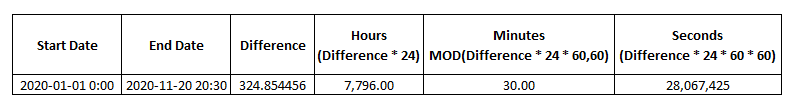
However, let’s assume that you also want to track seconds. We can do that as well. I’ll break out another column for seconds. There, I’ll multiply the difference by another factor of 60, to get the following:
I added 25 seconds to my end date, which is why you’ll notice there’s a slight change in the difference column from this screenshot and the earlier one. Right now, total seconds tells me there are 28,067,425 seconds between these two times. If I want to get the raw number of seconds, then I’ll again use the MOD function and again use 60 as a divisor, since now I want to factor out the minutes:
I now have a clean breakdown between hours, minutes, and seconds between these two times. But if you want to calculate more than just hours between two times, you can also incorporate the number of days as well.
Breakdown of days, hours, minutes, and seconds
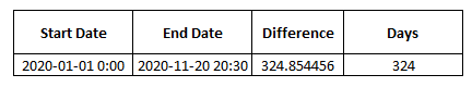
If I wanted to take a different approach and break the difference down by days, and then by hours, minutes, and seconds, I’ll first need to break out the days. Since that’s the default calculation for Excel, all I need to do is use the ROUNDDOWN function on the difference. The formula is as follows:
=ROUNDDOWN(difference,0)
And that gives me this:
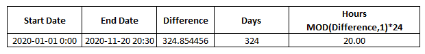
If I wanted to get the hours that are remaining, what I can do is take the difference, use the MOD function, but this time I’m using a divisor of just 1, since I really only want the decimal place after the full number. Then I’ll multiply that by 24 hours, and again, use the ROUNDDOWN function:
=ROUNDDOWN(MOD(difference,1)*24,0)
Now my hours total looks like this:
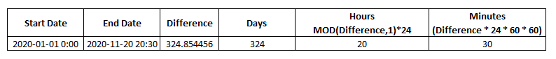
I’ve got a nice round 20 hours, which makes sense since 8:00 PM is 20:00 on a 24-hour clock. To calculate the difference in minutes, I can revert back to the earlier calculation where I used the MOD function to determine what’s left over after multiplying the difference by 24 and 60, and then dividing it by 60 minutes:
The seconds calculation will work the same way as well. The only difference in the way to break out hours and days was to adjust the hours calculation to ensure it isn’t taking in the full hour difference, only the residual amount that pertained to the current day.
Now that you’ve got all the chunks broken down between days, hours, minutes, and seconds, you could concatenate that into one large formula, Something like this might work:
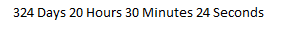
=CONCATENATE(daydifference,” Days “,hourdifference,” Hours “,minutedifference,” Minutes “,seconddifference, ” Seconds”)
That produces the following:
For this not to be a messy result, you’ll want to ensure you’re using the ROUNDDOWN function in each of those calculations so that you aren’t keeping any trailing numbers.
If you liked this post on how to calculate hours between two times, please give this site a like on Facebook and also be sure to check out some of the many templates that we have available for download. You can also follow us on Twitter and YouTube.
An amortization table is a useful tool when you need to calculate interest payments, principal payments, and to track the balance that’s owed on a loan. However, you don’t have to create a full schedule to get these values and below I’ll show you two functions that can get you that information quickly and easily. First, let’s start with what a typical amortization schedule looks like.
Creating the amortization schedule
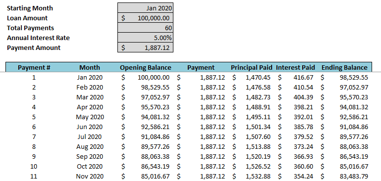
When you set up an amortization schedule, you’ll track the balances, interest, and principal payments. It often looks something like this:
You could use the table to determine what the balance is at the end of period 10 or to add up all the interest payments up until that point. However, there’s another way to arrive at those totals, and that’s using two functions that are available in the newest version of Excel: CUMIPMT and CUMPRINC.
Using the functions
In the amortization schedule, we can see that the ending balance of the $100,000 loan by the end of period 10 is $85,016.67. We can use the CUMPRINC function get to that total as well. The function takes on the following arguments:
To calculate the cumulative principal payments, I’ll enter the formula with the following arguments:
=CUMPRINC(0.05/12,60,100000,1,10,0)
This gives me a total of -$14,983.36. When added to $100,000, it nets out to a balance of $85,016.64 — within just a few cents of the amount on the amortization table. The function gives you the flexibility to specify which periods you want to extract and so you aren’t limited in just tabulating the totals for the first 10 periods or starting from the beginning. You can start from period 13, or the second year, and so on.
If you want to calculate the total interest payments, then that’s where you can use the CUMIPMT function. It has the same arguments as the CUMPRINC calculation, so the formula will look very similar to what’s above:
=CUMIPMT(0.05/12,60,100000,1,10,0)
This tells me that the cumulative interest payments during the first 10 payment periods is $3,887.87. This matches what I would get by adding the interest payments in my amortization table over the same period, this time to the penny.
Should you use these functions instead of an amortization table?
On older versions of Excel, you won’t have access to these functions but if you’re using Microsoft 365 or Excel 2019, then these functions are available and can potentially serve as replacements for an amortization table. Now, if you need the table for audit purposes it may not be possible for you to do without an amortization table completely. But if you’re only generating the table just to determine how much you’ve spent on interest or what your balance will be at some point in the future, then these functions can certainly replace doing a full-blown amortization table.
If you liked this post on 2 Excel functions that can eliminate the need for an amortization table, please give this site a like on Facebook and also be sure to check out some of the many templates that we have available for download. You can also follow us on Twitter and YouTube.
Are you entering multiple lines of text in Excel and want to break it up into multiple lines? You don’t have to adjust the cell size to do it and below I’ll show you some ways that you can manage cells that contain a lot of text, including how to make a line break in Excel.
Creating a line break
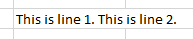
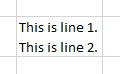
Here’s an example of a cell that could use a line break:
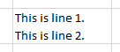
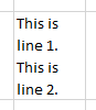
Currently, this bleeds onto where the start of the next cell should be. But rather than adjusting the length of my cell, I can position my cursor right after the period and before the ‘T’, hit ALT+ENTER, and now my cell looks like this:
Please note that if you want to create another line, you can’t just click on the cell and enter ALT+ENTER, you actually need to be inside the cell entering in values. To get into edit mode you can either click into the formula bar with the cell selected or click F2. Then, it’s a matter of selecting where you want to insert the line break. In the above example, the optimal position is just before the start of the second sentence. Then, once you’re there, you’ll click ALT+ENTER to move the following text down a line. You can repeat these steps to create as many lines as you’d like.
When creating an extra line, Excel automatically expands my cell vertically and selects the option to Wrap Text which is on the Home tab:
Using the ALT+ENTER shortcut tells Excel that you want to wrap your text and create a new line, which is what I’ve done in this example. Once wrap text is selected, your data will automatically conform to its cell size; the contents won’t bleed over into adjacent cells. For example, if I shrink my cell size then it no longer goes into the next cell, it just simply doesn’t show up:
If I were to double-click and auto-fit the column, then my cell would expand horizontally to accommodate the contents:
However, if I were to double-click on the row and use auto-fit there, then the row would get larger and then my cell looks as follows:
As you can see, once you’ve enabled Wrap Text, you don’t have to worry about your cell’s values moving into other cells. But at the same time, you may not necessarily want Wrap Text enabled for every cell since there’s the possibility that text gets cut off.
A good benchmark I normally use, especially for headers and where text may span multiple lines is to set the row height to 30. If that’s not enough, then I would at that point look at expanding the cell horizontally.
Another option that you have at your disposal if you want to accommodate a large value of text is to use Merge Cells. Generally, I’m not a big fan of merging cells because it can be problematic with formulas. But if you’re reserving this primarily for headers and text where there won’t be numbers in or near it, then it could be a practical alternative. That being said, I’d still keep this as a last resort.
If you liked this post on how to make a line break in Excel, please give this site a like on Facebook and also be sure to check out some of the many templates that we have available for download. You can also follow us on Twitter and YouTube.
In previous posts, I went over how to calculate the internal rate of return and how to discount future cash flows to arrive at a net present value. Today, I’ll go over another way you can evaluate projects, and that’s using the payback period. The payback period calculation is a simpler method than the other two approaches in that it just looks at how long it’ll take for you to recoup your money from an investment, or when you’ll hit breakeven.
Setting up the spreadsheet
To do this calculation, I’ll again use the discounted cash flow spreadsheet from my earlier example. The key difference in calculating the payback period is that you don’t need to worry about present value since this won’t take into account the time value of money.
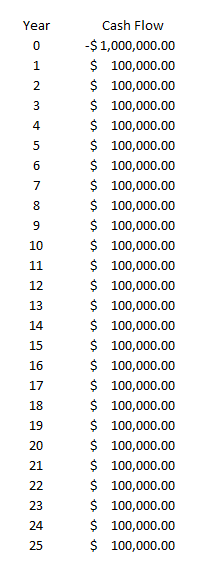
Let’s assume a scenario where you invest $1,000,000 into a project and generate cost savings of $100,000 every year. Here’s how that might look like over a 25-year period:
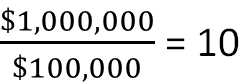
This is a really simple setup but let’s set up a formula to determine when the investment reaches breakeven. In this scenario, since the cash savings are always $100,000 every year, you can simply take the initial investment and divide it by the annual cost savings. The formula looks as follows:
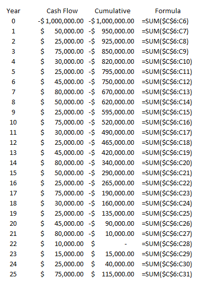
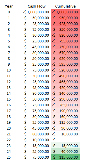
After 10 years, the investment will be paid back in its entirety and reach breakeven. If your cash flows will vary over the years, what you can do is use an average to try and smooth it out and get to an approximate payback period. Another alternative is to create another column that shows your cumulative savings or cash inflows and how much is left to reach breakeven. To calculate a cumulative sum, just use a regular summation formula but freeze the first cell so that your formula will always start from the same position. Here’s how you might set this up:
You’ll see that cell C6 is frozen as that’s where my first value is, and that’s where the $1,000,000 outflow of cash is. I’ve also changed my cash flows so that they’re different amounts each year, and under this scenario, you’ll notice that it’s not until year 22 that I reach breakeven. A better way to illustrate this is through conditional formatting, by highlighting the negative values and the positive ones in different colors.
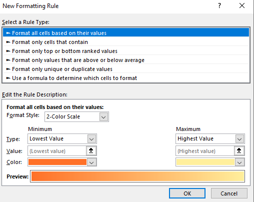
You can do this by selecting all the values in the cumulative field and under Conditional Formatting, selecting Format all cells based on their values, which gets you to this menu:
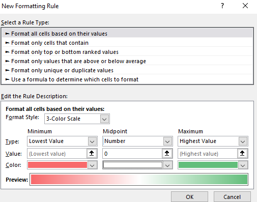
The first thing I’ll do here is to change the color scale so it shows three colors instead of just two. Then, I’ll set it up so that the lowest value is red, the midpoint is set to 0 and white, and the maximum is set to green:
Then, after clicking on OK, my values look like this:
Using the conditional formatting, I can easily see the progression of the red into white (breakeven), and then into green. It’s a lot easier on the eyes and allows you to quickly see the progress. If you want to look into more ways you can do this, check out this post on conditional formatting.
Payback period when factoring in time value
If you just want to calculate the payback period using a simple formula and your cash flow / savings is the same every year, then simply dividing your total investment by that amount will suffice. Then, it’s simply a matter of determining whether the number of years in the payback period is acceptable to you. If it is, you can move forward with the project. If the payback period is too far into the future, then you may want to re-consider it.
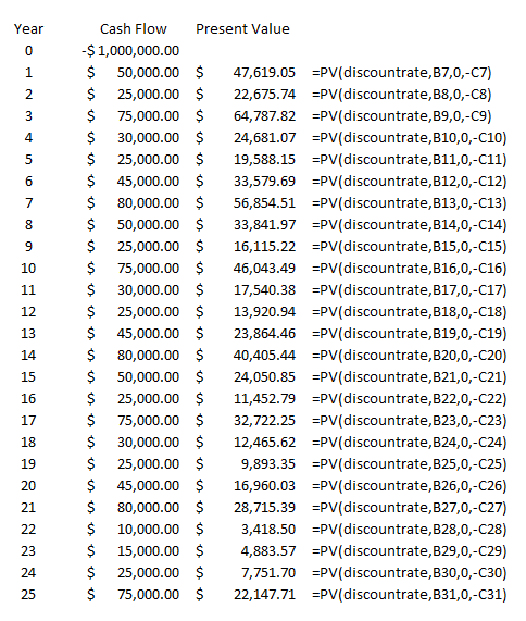
However, when you’re looking at a longer timeframe, you may want to consider incorporating discounted cash flow to give you a more realistic picture of the payout period over time. And while the typical payback period calculation doesn’t incorporate the time value of money, that doesn’t mean you can’t do it. In this example, I’ll calculate the present value of the cash flows like I did in the earlier post which looked at discounted cash. Using a discount rate and raising the cash flow to a negative power (years in the future), I can arrive at the present value. Here’s how that looks in an additional column, with the respective formulas off to the right:
Note that I used a named range for the discount rate. Column B relates to the Year field and Column C is the cash flow value in the future.
This time I use Excel’s built-in present value function, which requires you to enter the rate, the number of periods, payments (not applicable here), and the future value (which needs to be negative for this to calculate correctly). Using a 5% discount rate, I’ve populated the present values of each of the future cash flows.
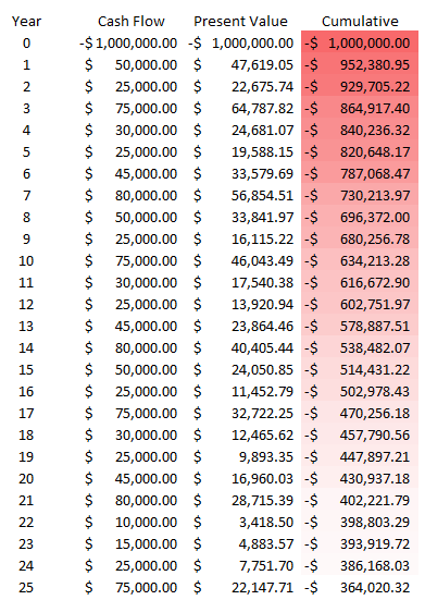
Now, I can add a column to track the cumulative values:
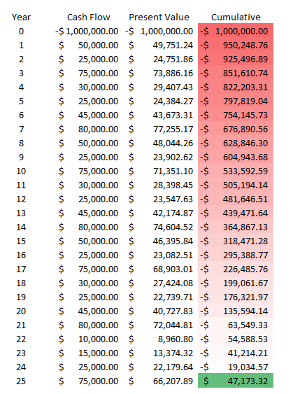
When factoring in the time value of money, my payback period is now well over 25 years. It’s an important reminder of just how important time value is. Under the previous payback period calculation that didn’t factor in the time value of money, the payback period was 22 years. In order for my payback period in this example to get to breakeven within 25 years, I’d have to set my discount rate to less than 1%. At 0.5%, this is what the schedule looks like:
Only after 24 years does the project attain breakeven in this situation, and that’s with a minuscule discount rate. Normally, in a payback period calculation, you’ll just stick to the investment total divided by the savings or cash flow that the investment will generate. However, there are significant drawbacks to doing so when it may take many years for an investment to breakeven. In that case, it may be worthwhile to consider the time value of money.
If you liked this post on how to calculate payback period in Excel, please give this site a like on Facebook and also be sure to check out some of the many templates that we have available for download. You can also follow us on Twitter and YouTube.