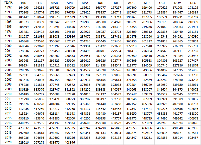
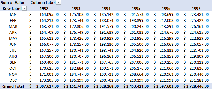
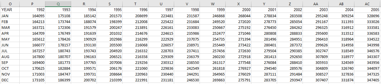
Often times, when you download a data table from somewhere it’s not in the format you need it to be. Tables are often in a summary format where you have months going down and years going across, or vice versa. It’s the end result of what you want a pivot table to look like, but you can’t easily turn that into a pivot table itself. Below, I’ll show you how to turn a summary table in Excel that looks like this:
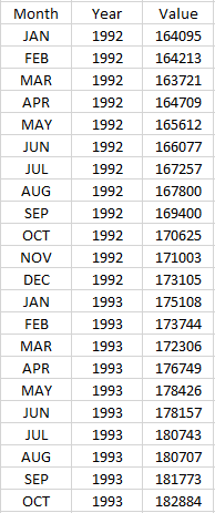
Into this:
This format is much more Excel-friendly and one that you can easily convert into a pivot table.
Converting the table
The data I’m using is the same one that I used in an earlier post that went over transposing data. Transposing data, unfortunately, isn’t enough to make data workable if you want to convert it into a pivot table. You’ll want data to be in a tabular format so that there’s a header for the month, year, and value.
You could manually transpose one year at a time and copy the data one by one. But of course, that isn’t optimal at all. The good news is I’ve got a macro that can help you flip that data in one click. It will go through the painstaking process of reorganizing the data for you.
Here’s the code for the macro. You can just put it into a module (I’ll leave a template to download below if you aren’t comfortable doing this step yourself):
Sub flipdata()

Dim cl, nxtcl As Range
Dim lastcol, lastrow, firstcol, firstrow As Integer


'get total number of rows and columns in range
lastcol = Selection.End(xlToRight).Column
lastrow = Selection.End(xlDown).Row

'get first column and row
firstcol = Selection.Column
firstrow = Selection.Row

'assign output starting point
Set nxtcl = Cells(lastrow + 2, firstcol)

nxtcl = "Header 1"
nxtcl.Offset(0, 1) = "Header 2"
nxtcl.Offset(0, 2) = "Value"

Set nxtcl = nxtcl.Offset(1, 0)


'cycle through data

For yr = (firstrow + 1) To lastrow

    For mth = (firstcol + 1) To lastcol

        nxtcl = Cells(firstrow, mth)
        nxtcl.Offset(0, 1) = Cells(yr, firstcol)
        nxtcl.Offset(0, 2) = Cells(yr, mth)
        Set nxtcl = nxtcl.Offset(1, 0)

    Next mth

Next yr

End Sub
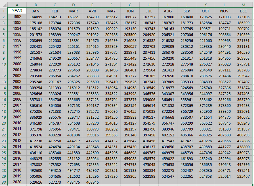
It will output the data a couple of rows below where your data ends. It’s important to select the entire range of data before running the macro since it will go through the range that you’ve selected, nothing else. And if there’s data below your selection, it will overwrite that.
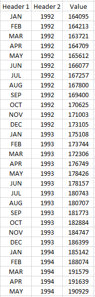
After you’ve selected the data, then you run the macro. In my template, I’ve got a button that you can press that will do the job for you and then you’ll get something that looks like this:
Once in this format, you can easily create a pivot table:
If you’d like to download the file that contains the macro, it’s available here.
If you liked this post on how to convert a summary table in Excel into a pivot table, please give this site a like on Facebook and also be sure to check out some of the many templates that we have available for download. You can also follow us on Twitter and YouTube.
It’s not often that you’ll need to transpose data in Excel, but when you do you’ll be happy to know how easy it is to do. In this post, I’ll go over not just transposing data but converting text to columns and showing you how you can change a block of text into data that you can use for analysis. After all, there’s no use trying to transpose data if it isn’t in a workable format.
If you want to follow along, the data I’m going to be using comes from the United States Census Bureau. In particular, I’ll be pulling the monthly retail and food services sales data for the past couple of decades. You can download that information here.
Copying the data into excel
Let’s start with the first step, and that’s to get the data into Excel. It’s in text, but the information is workable since it’s in the format of a table. I’m not going to copy the seasonal factors, I just want the raw, unadjusted sales numbers. To get the data into Excel, I’ll just highlight the sales data, copy it, and then paste it into a blank Excel sheet. Here’s how it looks:
The first thing that needs to be fixed is that everything is in column A. The data as it is won’t be useful for data analysis and needs to be cleaned up before it would make sense to try and transpose it.
Use text to columns to spread data across multiple columns
In Excel, there’s a Text to Columns button right on the Data tab that will help you to quickly and easily spread the data onto many columns. In our example, select column A and click on this button or something that looks similar to it if you’ve got an older version of Excel:
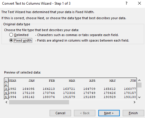
You’ll then see an option for how you want to break out the data. The default is Fixed Width:
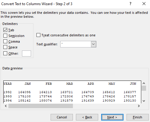
However, that’s not an ideal way to split the data and it rarely ever is. Unless the data is always the same length it won’t be very useful. At best, it’ll be time-consuming to get the output in the format that you’re after. Instead, change the option to Delimited. Click on Next, and then you’ll see various options for splitting the data:
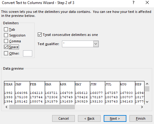
The data isn’t separated by a semicolon, comma, or any other distinctive character. There is, however, a space between each amount. That’s why we’ll want to unselect Tab and tick off the box for Space instead. We see a preview of how the data will be separated, which looks to be what we’re after:
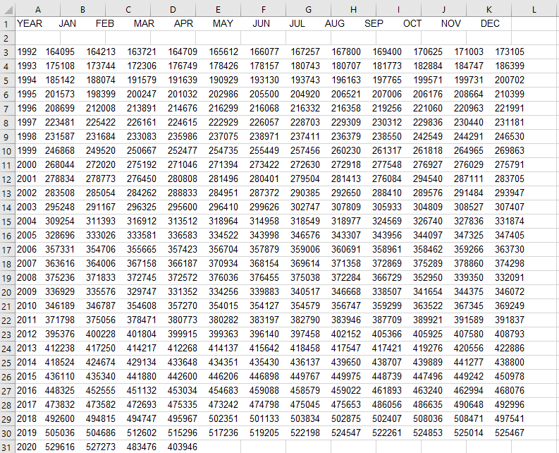
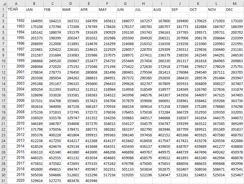
At this point we can just click the Finish button and our output will now look like this:
Now we’ve got data that’s much more usable as every number is in its own individual cell. The one thing we’ll want to do before we get to transposing it is to get rid of row 2. The blank row effectively separates the headers from the data, and that’s not ideal.
Next up, let’s get to the actual transposing part.
Transposing the excel data
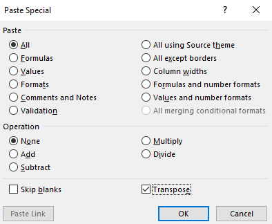
By transposing data, you’re flipping the rows and columns around. And to do that is pretty straightforward. First, copy the data, including the headers, and then click on a blank cell — I’m going to pick O1. Then, right-click and select Paste Special. There, you’ll see an option at the bottom that says Transpose:
Then your data will be flipped, or transposed. You can also select Transpose right from the Paste Special menu and select the icon from there. You can also use shortcut keys S and T to select the menu and then select the transpose button.
Now the data looks like this:
The years are now spread across the columns while the months are going down the rows.
Ultimately, whichever way you want to see the data comes down to personal preference. And by transposing it, you can change the view easily to make that happen.
If you liked this post on how to make a transpose data in Excel, please give this site a like on Facebook and also be sure to check out some of the many templates that we have available for download. You can also follow us on Twitter and YouTube.
A countdown timer can help you track how much time there’s left to do a task or until a deadline comes due. Below, I’ll show you how you can make a countdown timer in Excel that can track days, hours, minutes, and seconds. In order to make it work, we’ll need to use some VBA code, but it won’t be much. And if all else fails, you can just download my free template at the end of the post and repurpose it for your needs.
Let’s get right into it and start with the first step:
Calculating the difference in days,
To calculate the difference between two dates is easy, as all you’re doing is subtracting the current date and time from when you’re counting down to.
The start date is just going to be today, right this very second. And Excel has a convenient function just for that, called NOW. It doesn’t require any arguments and all you need to do is enter the following formula:
=NOW()
Entering the date and time you’re counting down to is a bit trickier. As long as you enter it correctly, then calculating the differences will be a breeze. However, this may involve a little bit of trial and error since it’ll depend on how your regional settings are setup. For the countdown date, I’m going to set it to the end of the year. Let’s say 11:00 PM on New Year’s Eve. Here’s how I input that into my spreadsheet:
2020-12-11 11:00 PM
The key things to remember here are that there should be a space between the time and the AM/PM indicator (if you use it) and there should be two spaces between the date and the time. Then, it’s just a matter of whether you’ve got the right order of date, month, and year. This is where you may need to do some testing on your end to ensure you’ve got the correct order.
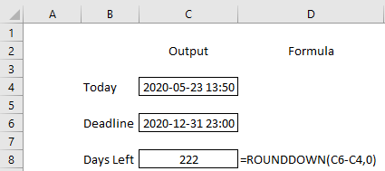
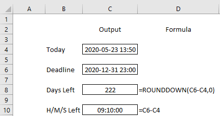
Now that the dates are set up, we can calculate the difference in days. To do this, we can just calculate the difference and use the ROUNDDOWN function to ensure we aren’t adding partial days:
There are 222 days left until the end of the year. By using the NOW function, the formula will automatically update and tomorrow the days remaining will change to 221, and so on. If your output’s looking a little different, make sure to check the formatting and that it’s set to days.
Calculating the difference in hours, minutes, and seconds
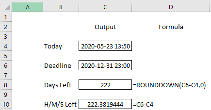
There’s not a whole lot of complexity when it comes to calculating the difference in hours, minutes, or seconds. We’re still subtracting the current date from the deadline. The only difference is that now we’re just going to change the formatting. If I do a simple subtraction, I end up with a fraction, which isn’t really usable in its current format:
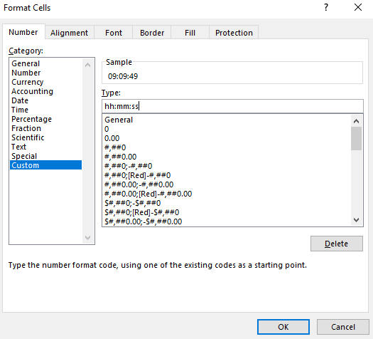
The trick here is to change the format of this cell so that it shows me hours, minutes, and seconds. And that’s an easy fix. If I just click on cell C10 and click CTRL+1, this will get me to the Format Cells menu. In here, I’ll want to select a Custom format so that the cells just shows hours, minutes ,and seconds:
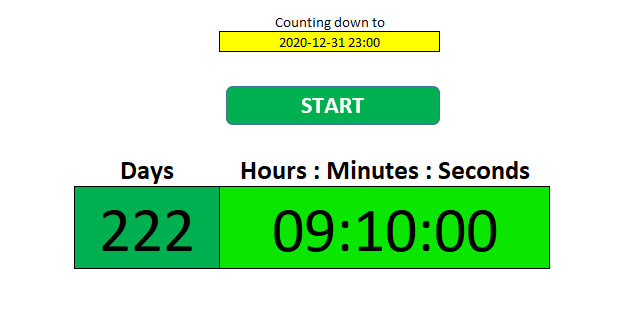
Here’s what the countdown timer looks like after the format changes:
It’s important to include a date in the calculation even though we’re just doing a difference between hours, minutes, and seconds. Otherwise, the formula wouldn’t correctly calculate in all situations, such as when the deadline hour is earlier than our current hour.
Putting it all together
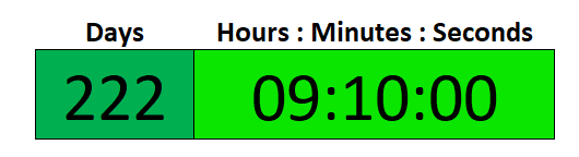
Now that all the calculations are entered in, now it’s just a matter of formatting the data. We can create a countdown clock that separates days remaining, from hours, minutes, and seconds remaining.
One cell can have the difference in days, while another will have the difference in hours, minutes, and seconds. This goes back to just modifying the formatting and applying a custom format. Here’s how mine looks:
Although we’ve gotten to this point, the challenge is that this countdown timer still doesn’t update on its own. Unless you want to click on the delete button all the time, the countdown isn’t going to move unless there’s something to trigger a calculation in Excel. That’s why we’re going to need to add a macro to help us do that, which bring us to the important last step of this process:
Adding a macro to refresh every second
We need a macro to update the file. Whether it’s every second, every five seconds, it’s up to you. While the countdown timer will update when someone enters data or does something in Excel, that’s not much of a countdown. This is where VBA can help us. If you’re not familiar with VBA, don’t worry, you can just follow the steps below and copy the code.
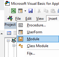
To get into VBA, click on ALT+F11. From the menu. Once you’re there, click on the Insert button on the menu and select Module:
Over to the right, you’ll see some blank space where you can enter in some code. Copy and paste the following there:
Sub RunTimer()

    If Range("C10") <> 0 Then
        Interval = Now + TimeValue("00:00:01")
        Application.Calculate
        Application.OnTime Interval, "RunTimer"

    End If
End Sub
One thing you may to change is the reference I made to cell C10. Change that to where you have your countdown timer. As long as there’s a value in the cell, the macro will continue running. All it does is check if there’s a value there, and if there is, it updates the worksheet every second. And by doing that calculation, your countdown timer will update even if you’re not making any changes to the spreadsheet.
You can also change the interval which currently updates every second, as noted by the 00:00:01. You can change this to five seconds, 10 seconds, however often you want it to update.
But there still needs to be something that triggers the macro to start running. You can assign a button or shortcut key to do that.
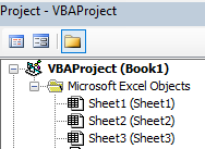
However, in this example I’ll activate it when the sheet is selected. Inside VBA, you should see a list of worksheets. Double-click on the one that contains your countdown timer:
You’ll again see blank space to the right where you can enter code. And you’ll also see a couple of drop-downs near the top that you’ll want to look for. By default, the first one should say (General). Change this to Worksheet:
Next, change the other drop-down which will probably say SelectionChange. Change it to Activate. Then you should see something like this:
Copy the following code into there to call the macro we created above:
RunTimer
Now when you switch to another worksheet and come back to the current one you’ll notice your countdown timer is updating on its own. If you want it to stop it, just clear the cell that has the timer. Otherwise, the macro will continue running every second.
The Countdown Timer Template
If you’d rather just use a template, then you can download one that I’ve made here. You don’t have to worry about macros and instead you just need to enter the end time; the time that you’re counting down towards.
I’ve also got a start/stop button that you can toggle to get the countdown timer going and that will pause it:
You can move the button as well as the time your counting down to onto another sheet if you don’t want someone altering it. If you have any questions or comments about this template, please send me an email at [email protected]
If you liked this post on how to make a countdown timer in Excel, please give this site a like on Facebook and also be sure to check out some of the many templates that we have available for download. You can also follow us on Twitter and YouTube.
If you’ve got a large data set, you know how important it is to be able to filter that data quickly and easily. Knowing how to filter efficiently in Excel can make it easy to not just pull up the data you need, but to also run calculations. Below, I’ll show you multiple ways that you can filter data.
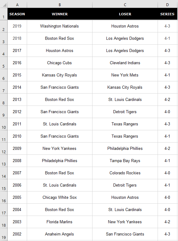
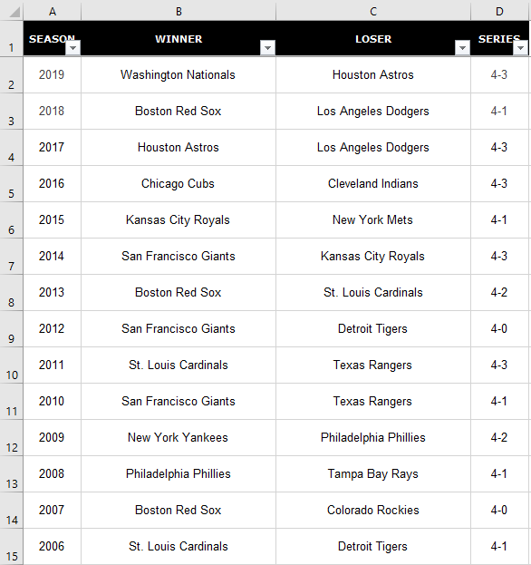
For this example, I’m going to use a list of all the MLB World Series champions and runners-up.
Using the auto filter
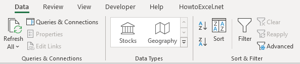
A quick way to filter the data is by using Excel’s auto filter. To enable it, click anywhere on the data set and click on Filter button from the Data section:
Clicking the button will create drop-down buttons that you can now use to filter the data with:
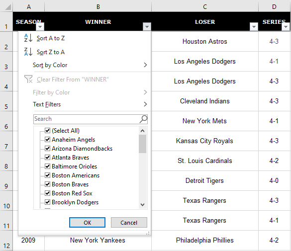
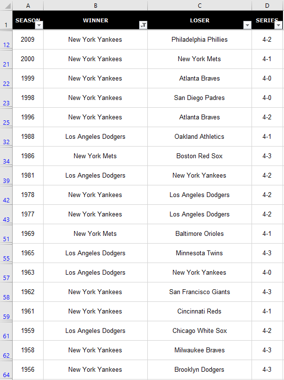
Suppose I wanted to see all the times that the New York Yankees have won. To do that, I would click on the drop-down button in the Winner column, where I’d now see all these options:
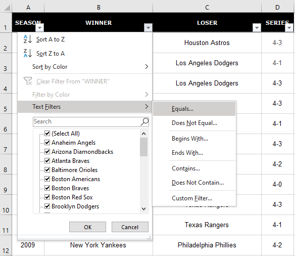
Filtering in Excel can be as easy or complicated as you want it to be. You’ll notice there’s even an option to Filter by Color that’s been greyed out since I don’t have any colors in my data set. If I click on the Text Filter option, I’ll have more options to choose from. I can look for partial matches and I can select an exact match as well:
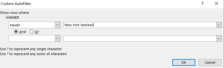
In the following screen, I’ll enter in New York Yankees as my search term:
I can also have multiple criteria. For instance, I could say I want to see any victories by the New York Mets as well. In that case I could just enter another criteria and enter their name. However, there’as an even easier way to do that.
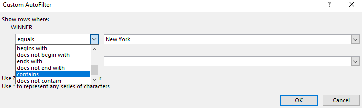
Although in the criteria, equals is selected, I can change that by clicking on the drop-down, and there I’ll have more choices:
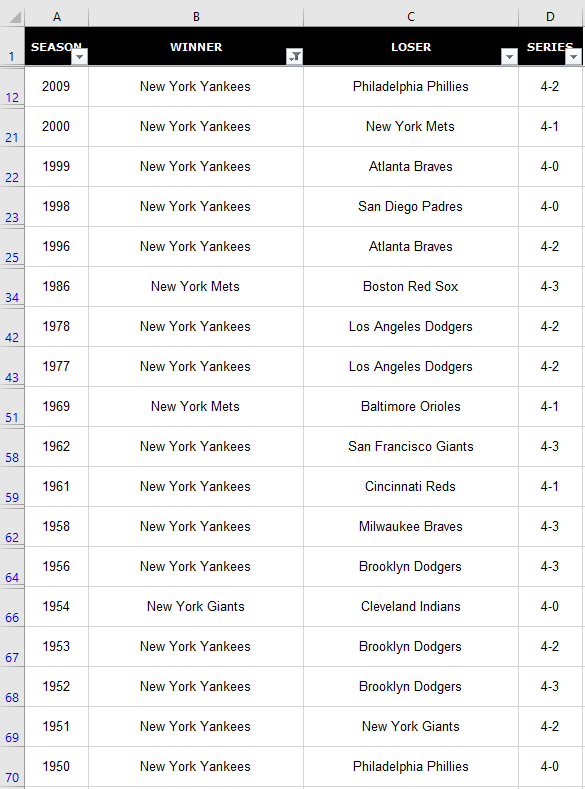
I can select contains and just change the search criteria to New York. So even though I selected equals as my initial match criteria, I don’t have to worry about sticking to it. When I click OK, I now see my list of titles won by any team that had ‘New York’ in their name:
Not only do we have the Mets and Yankees on this list, but there’s also the New York Giants.
You’ll notice that the row numbers on the left are now in blue. This is how you can tell that your data is filtered. And so if you’re looking at your data set one day wondering why you’re missing information, have a look at the row numbers, as they may tell you the data’s filtered. If you want to unfilter the data, go back to the Filter button and click it again. Then your data set will be unfiltered and the drop-downs will be gone.
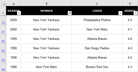
What you can also do is select the individual drop-down and clear the filter. You can tell which column has a filter in place by looking at the drop-down. In the Winner tab, the button shows a filter icon:
Clicking on that drop-down I’ll have the option to eliminate the filter:
Clicking the Clear Filter From “WINNER” button will now reset the filter and keep the drop-down buttons in place.
Filter using selections
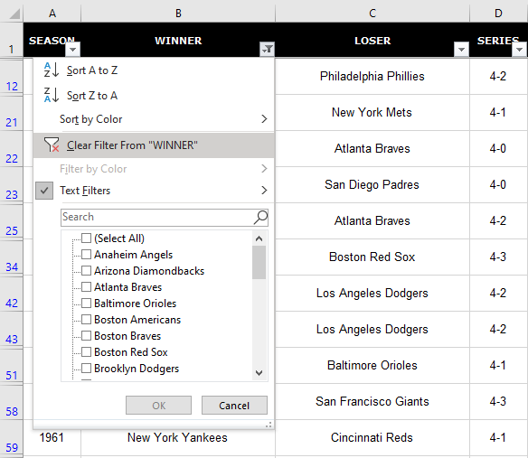
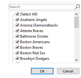
Using the text filter isn’t optimal because on newer version of Excel you see the list of items that you can choose from:
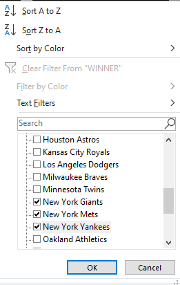
If I uncheck Select All and then scroll down to the New York teams and select them, I’ll arrive at the same result as if I did the text filter earlier:
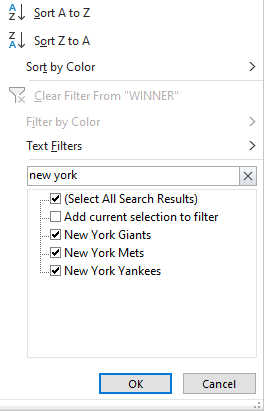
However, even this isn’t optimal. If I’m looking for a partial match, then I can just type in ‘New York’ in the search field and it’ll get the same selections:
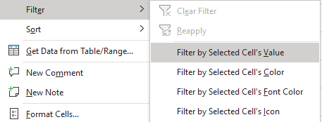
There’s another less common way that you can filter data. If you’re just looking for one match, you can right-click on the value that you want to filter. Then, right-click on it and click Filter by Cell’s Value:
With this method, the drop-downs in the headers don’t have to be enabled. Once you run this filter, they will be there, however.
Filtering multiple combinations
It’s easy to filter when the names are similar. But if I wanted to filter the data for anytime a team from New York, Chicago, or Los Angeles has won, then it gets a bit trickier. One method would be to go back to the text filters and run multiple filters. But that’s an antiquated way of doing it. However, if you’re running an older version of Excel, that may be your only option.
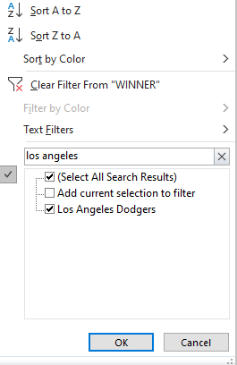
If you can search through the filter, then there’s an easier way for you to do this. First, let’s go back to searching for ‘New York’ in the filter. We’ll again have all the New York teams in the list.
Next, let’s go back to the drop-down and search again. This time for ‘Los Angeles’ but before clicking OK, we’ll want to click off the box that says Add current selection to filter:
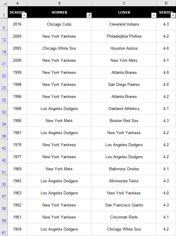
By default, this option isn’t checked. If I were to just click OK, the filter would be a list of Los Angeles teams only. But by checking off that box first and then clicking OK, I now have a list that contains both Los Angeles and New York:
After repeating the process for Chicago I’ve now got all three cities in my list without having to go through the text filter:
Use subtotals to make your filters even more useful
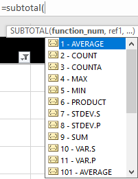
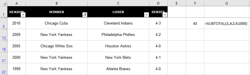
If I wanted to run a quick tally to see how many of the teams I’ve filtered have won a championship, I could use a COUNTIF function and enter their names. But if you want something more flexible where you can quickly run the filters as I’ve done above and see how many teams are in that list, you can use the SUBTOTAL function. The function takes in an argument for what type of calculation you want to do.
Now, since this data isn’t numeric, I’m going to use a COUNTA function, which is function number 3. For the range, I can use any column since it doesn’t matter which one I’m counting. But I will use range A2:A1000 because I don’t want to include the header in my total. Here’s how my formula looks like:
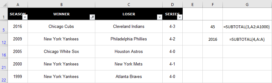
I could also use the MAX function to see the last time one of the teams I’ve selected has won. I’ll put that directly below the other formula:
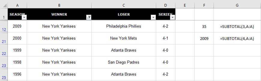
Now, if I were to re-filter this data, this time, only for New York, my subtotals will automatically update:
The benefit of using the SUBTOTAL function is your data updates along with your filters. If you want the data to be static and not change, that’s when a regular COUNTIF function would be more appropriate.
If you liked this post on how to filter in Excel, please give this site a like on Facebook and also be sure to check out some of the many templates that we have available for download. You can also follow us on Twitter and YouTube.
If you’ve inherited or downloaded a data set, you know that sometimes you’ll need to combine data together to make it in the format that you want. A good example is a list of addresses where you may have the street information in one column and the zip or postal codes in another column. To get all the information in one cell would require combining the information. Below, I’ll show you multiples ways of how you can combine two or more columns in Excel.
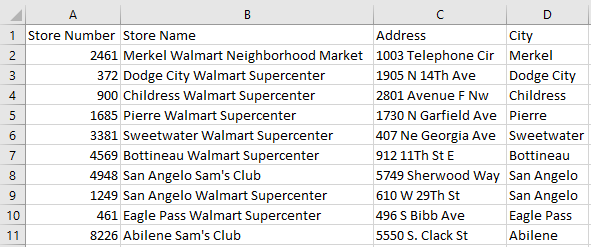
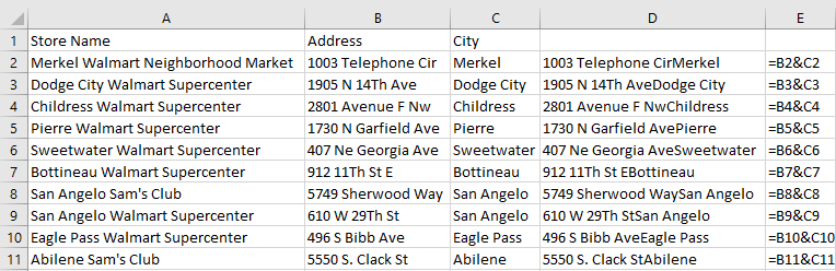
My data set for this example includes some sample address information on Sam’s Club and Walmart locations in the U.S. :
Using the ampersand to combine columns together
The easiest way is to join the cells through a simple formula. The easiest way to do so is by using the ampersand (&). In column D below, I’ve joined the cells and in column E is the formula that I’ve used:
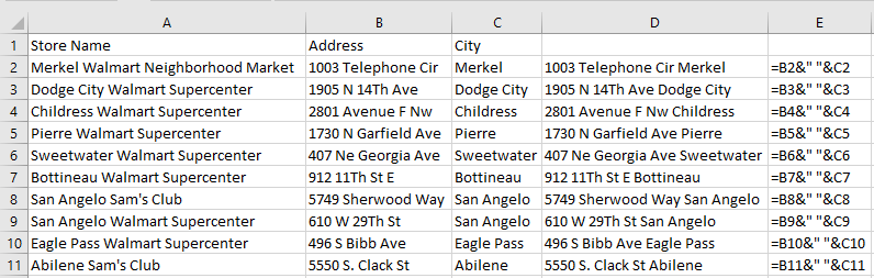
This gets the job done but you’ll notice a small issue: there isn’t a space between the information. that makes the data a bit messy and it’s probably not what you want. But it’s an easy fix. It can be addressed by adding another ampersand between the cells and add open quotes ” ” to add a space. This is how my spreadsheet looks after I’ve made those changes:
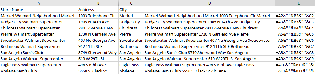
This can be expanded to more than just two columns. If I wanted to add the store name field (column A) into the mix, then it’s just simple as adding another ampersand for the field and another one for another extra space. Here’s how the data looks like all three columns joined together:
This can start to become a bit cumbersome as you add more fields into one cell. An alternative way that you may find easier if you’re working with several columns is using the CONCATENATE function.
Using the CONCATENATE function
The CONCATENATE function works very similar to how the ampersand. However, it’s a bit cleaner in that you don’t have several ampersands in your formula. If you wanted to group cells A2, B2, and C2, your formula would look like this:
=CONCATENATE(A2,B2,C2)
If you want a space to be included between each of those fields, then it looks like this:
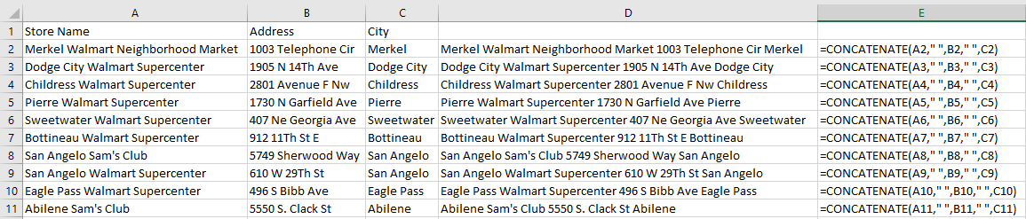
=CONCATENATE(A2,” “,B2,” “,C2)
Here’s how that would look if I applied it to my existing data set:
You can use commas to separate the data if you prefer and in that case, you would just use “,” instead of an empty quote. You can also add extra spaces in between quotes to space out your data even further.
But whether you choose to use the ampersand or the CONCATENATE function just comes down to preference. Either approach can get the job done.
If you liked this post on how to combine cells in excel, please give this site a like on Facebook and also be sure to check out some of the many templates that we have available for download. You can also follow us on Twitter and YouTube.
Whether you’re tracking sales or costs in excel, it’s important to capture not just your monthly totals but your cumulative year-to-date amounts as well. And to do that in excel, you’ll need to calculate a cumulative sum. Ideally, you’ll want to see a current month’s total alongside the year-to-date figure. Below, I’ll show you how to do that as well as how to make cumulative totals work with multiple years.
Calculating the current month and cumulative sums
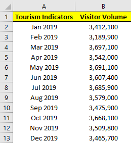
First thing’s first, let’s start with a data set. This time around, I’m going to pull the monthly tourist information for Las Vegas. This year, that could prove to be interesting given the impact of COVID-19 on tourism in the city. Here are what the numbers looked like for 2019:
If we wanted to calculate the total visitor volume it would be as simple as the following formula:
=SUM(B:B)
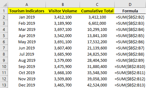
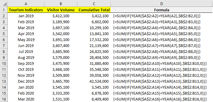
However, if we want the cumulative totals then we can’t just grab the entire column. Instead, we’ll need to add another column that has the cumulative amounts for each month. The formulas will still involve the SUM function but they will need to be from January up until the current row. Here’s what the formulas look like:
The formulas for column C are shown in column D. The key here is freezing the first cell (B2) so that as you copy the formula down in C2, it won’t move while the other cells will.
Calculating cumulative values isn’t too complicated, but it’s a bit trickier when your data set spans multiple years.
Calculating the cumulative sum when working with multiple years
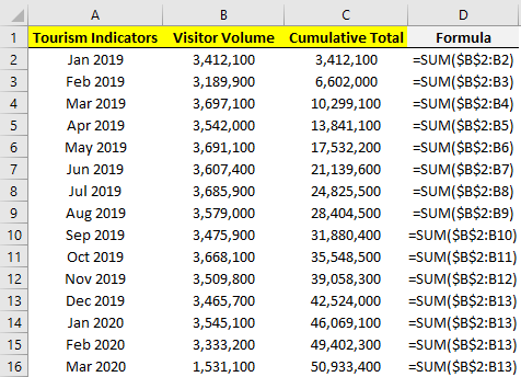
The above scenario works well if you have just one year. But it won’t work if you decide to add next year’s data without resetting the formula. Here’s how it would look if we added the 2020 data:
As you can see, it just keeps on adding on to the previous year’s data, which is not what we want.
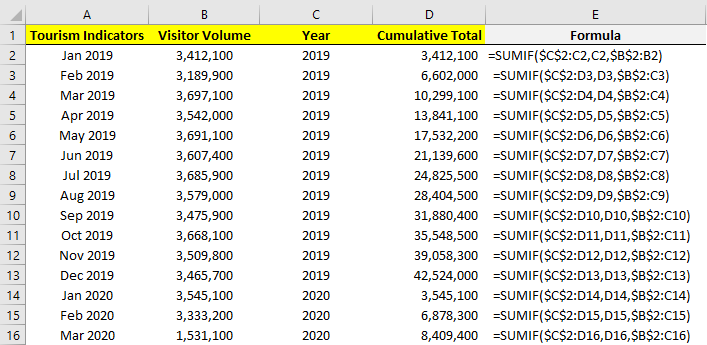
There are multiple ways that you can calculate the cumulative sum per year and so that the calculation resets on its own. Let’s start with the easiest route: adding an extra column for the year. Using the YEAR function we can extra what the year is in column A. Then, rather than using the SUM function, we will use the SUMIF function to do the cumulative count, but only if the year is the same:
The logic similar to the earlier formula, we’ve just added a condition where the year in column C has to match the year that specific row belongs to. That’s why once we hit 2020, it resets. For this to work, we still need the months to be in order.
Another way that you can calculate the cumulative total without a helper column is by using an array:
We need to evaluate every cell to see if it relates to the correct year, and if it does, it gets included in the range to sum. The array allows us to do two calculations in one: an IF calculation embedded within a SUM calculation which doesn’t require the helper column.
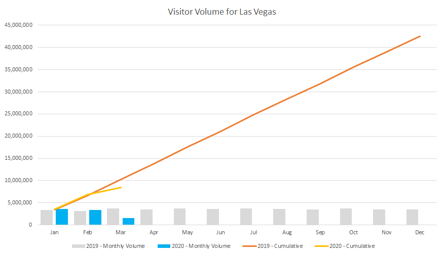
A big advantage of having multiple years on your data set rather than separating them out is then you can put them into a pivot table and create a pivot chart that helps plot both of them:
From this, we can see that there was a sharp drop off in March due to the outbreak of COVID-19 and that the cumulative figures are now well under 2019’s numbers. By having both cumulative and monthly totals available, we can display them both on one chart that helps to summarize the information quickly and easily.
If you liked this post on How to Calculate Cumulative and Year-to-Date Totals in Excel, please give this site a like on Facebook and also be sure to check out some of the many templates that we have available for download. You can also follow us on Twitter and YouTube.
Scroll further down if you would like to see details as to how this calculator works and a description of it.
There is a new version of this calculator available here (mobile-friendly) that will make calculations at multiple price points at once (use the new interval field to specify how much in price you want to jump by). It will also let you know how low you can average down at the current share price.
If you invest in stocks and want to know how much it would cost you to average down, this calculator will help you do just that. Averaging down is a great way to take advantage of a stock that’s dipped in value and that you’re confident won’t stay there. By purchasing more shares of a stock at a lower price, you’re bringing down the average cost of your total investment. And that means you’ll need the stock to rise to a lower price than before to turn a profit. Or if you’re already in the black, then you can put yourself in a great position to increase those profits.
How the average down calculator works
To use this calculator, you’ll need to enter the total dollars that you’ve invested in a stock, how many shares of it you own, what the current price of the stock is today (or the price that you plan to buy it at), as well as what price you want to average down to. Then, click on the Calculate button. The calculator will then tell you how many shares you’ll need to buy and how much it will cost you in order for you to get to that average.
Note that since you can’t average down below what the current share price is, you’ll have to make sure that your desired average price is higher than where the stock is today. Here is the calculator:
If you liked this free average down calculator, please give this site a like on Facebook and also be sure to check out some of the many templates that we have available for download.
A word search can be a great way to pass the time and for kids, it can help them practice their spelling as well. With this free word search maker, you can easily create a random new word search in just seconds. With small, medium, and large sizes to accommodate different ages and skillsets, the template provides a lot of flexibility. You can download it here.
Let’s jump right into it and see how the template works:
How to create a word search using the template
There are three tabs in this template: WORDSEARCH, WORDSEARCH.MED, and WORDSEARCH.SM. They indicate their size and difficulty. If you want to create something fairly simple, then the small (SM) tab will work best and it can accommodate up to 10 words. The medium (MED) tab is a bit bigger and you can have up to 15 words. And the main tab will allow you to plot up to 20 words.
Below the actual word search, you’ll have a list of spaces where you can enter your words in, titled Word List:
Each list contains a pair of boxes. The small one off to the left is where you might tick off that a word has been found. The larger box on the right is where you will enter the actual word.
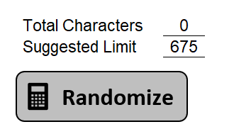
Further off to the right, you’ll see how many characters your words have taken up as well as a suggested limit:
If you’re over the suggested character limit then the macro may have trouble finding space for all your words. If that happens, you’ll get an error message saying so. However, you can still try and see if it’ll work. to create a new word search, click on the Randomize button shown above. This will plot your words randomly in every possible direction, up, right, left, down, and diagonally as well.
Once the words are plotted, then the remaining spaces will be filled in with random letters. However, not every space will be a random mix of any possible letter in the alphabet. Less common letters like Z, X, and Q won’t have the same odds of showing up as more common letters. This is done in order to make the word search more challenging.
When the word search is entirely populated you can just print it off. You won’t see where the words were plotted on the word search without actually searching for them yourself. So if you wanted to create a word search for yourself, that’s entirely possible as even the person who runs the macro won’t have any advantage of knowing where the words were placed.
If you liked this free word search maker template in excel, please give this site a like on Facebook and also be sure to check out some of the many templates that we have available for download. You can also follow us on Twitter and YouTube.
Creating charts and graphs is a great way to display data visually and make it easier for users to read and understand it. However, in some cases, you don’t want or need a big chart, and something smaller would be more useful. This is where sparklines can come in to play and help you get your point across without a big chart in the way. Below, I’ll show you how to quickly and easily make sparklines in Excel that can quickly add context to your data.
*Please note that sparklines were a new feature of Excel 2010. If you’re running an older version of Excel, you won’t have these options available*
Getting the data set ready
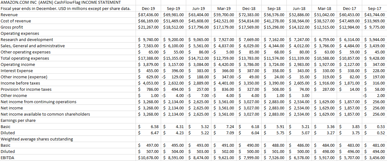
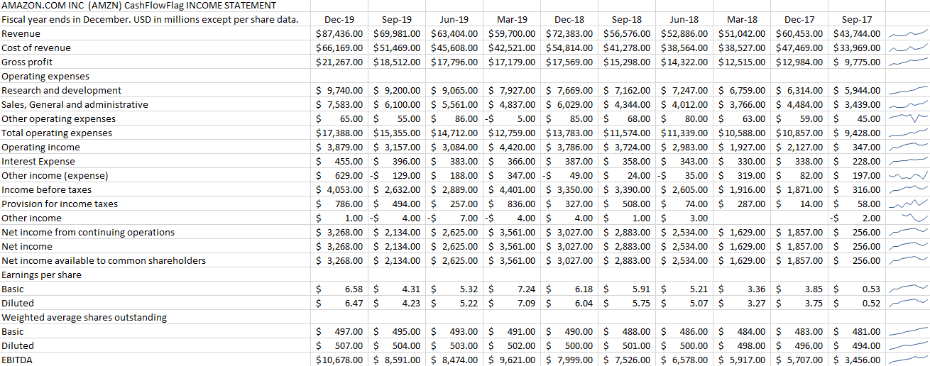
I’ll show you how to create sparklines using my data, which is a download of Amazon’s income statement over the past 10 quarters. Here’s what it looks like:
From afar, it’s not the easiest thing to analyze to identify any trending. And ideally, we’d like to have some trending shown for each major income and expense category. Adding a chart just isn’t useful in this case, and this is where sparklines can help.
Creating sparklines in just one click
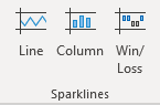
I’ll start by selecting the row that has revenue and then on the Insert tab and under the Sparklines category I’ll select the Line button:
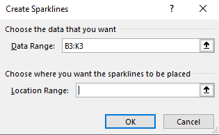
It will then show me the range that I’ve selected and it will allow me to select where I want to place my sparklines:
In most cases, you’ll probably want this right next to your data. And that’s what I’m going to do — put it in the next cell to the right of the data, L3. Now it’s created my sparkline:
But there’s just one problem:
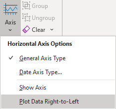
The sparkline is showing a downward trend. Amazon’s revenue has been increasing, not decreasing. One solution is to re-arrange my data, but that’s not necessary. To fix this, I select the sparkline and then under the Sparklines tab I click on Axis and select the option that says Plot Data Right-to-Left:
Now my sparkline looks a lot better:
This is an optional step and it depends on which direction you want your sparkline to go in.
Applying sparklines to other rows
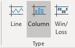
Now that I’ve got one sparkline setup, it’s time to set up the sparklines for the rest of the income statement line items as well. Surprisingly, this is as easy as just dragging the sparkline down and copying it down to the other rows:
One of the cool features of sparklines is you can quickly add trending to every item without having to add a separate chart or graph for each row. And even for the rows where there was no data, it doesn’t result in an error, either.
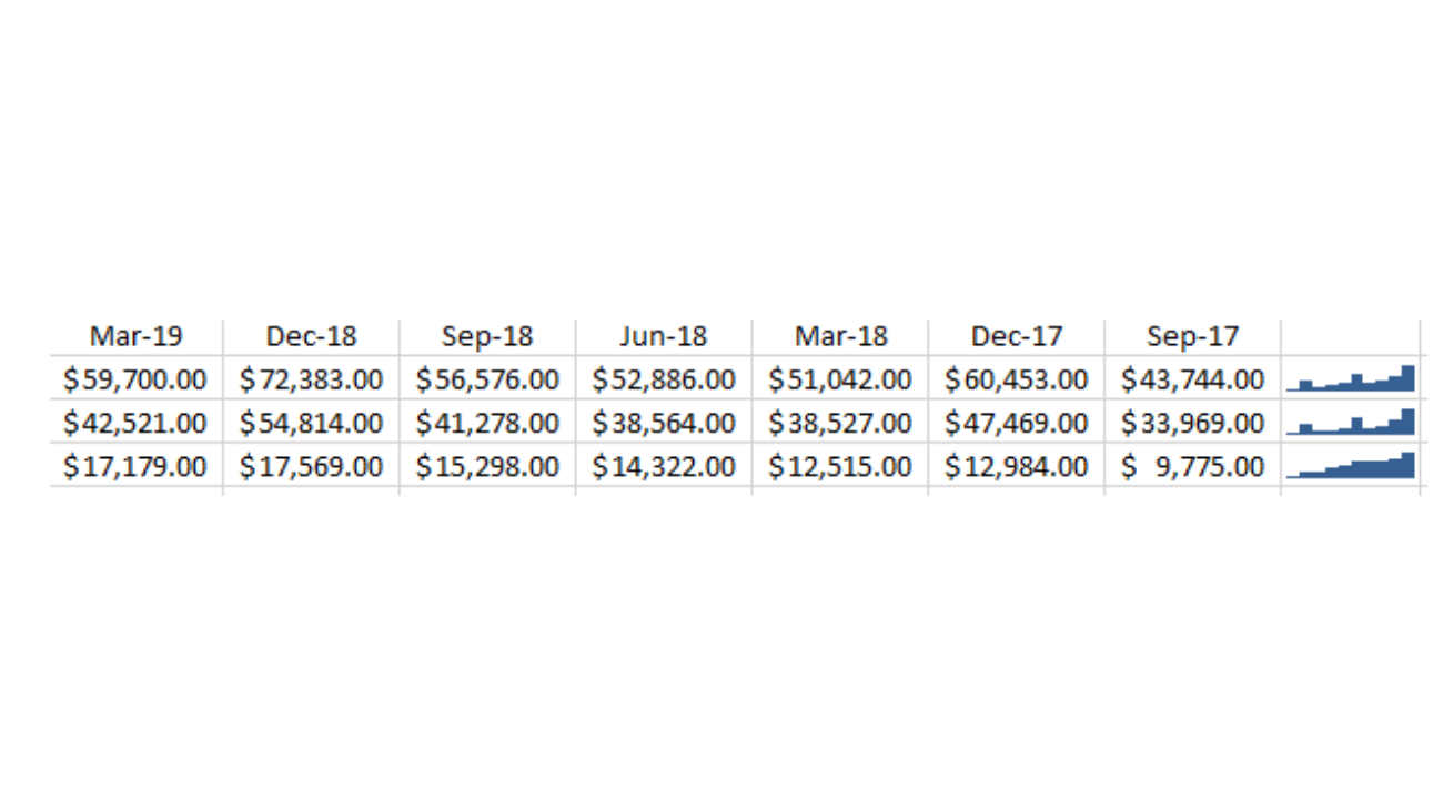
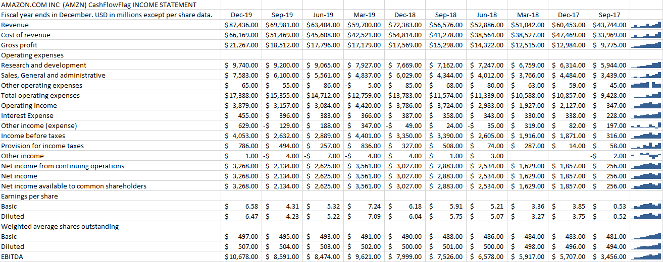
If you prefer a column chart to a line chart, then you can easily make the change as well in the Sparklines menu:
It will quickly change the format of the charts:
There’s also a win-loss chart that you can use if you have negative and positive values. However, in most situations, you’re going to use either line or column charts, especially when you’re looking to show trending. But
You can change the color and other features of the sparklines just like with other charts. And all those options are available from within the Sparklines tab.
If you liked this post on how to create a drop-down list in Excel, please give this site a like on Facebook and also be sure to check out some of the many templates that we have available for download. You can also follow us on Twitter and YouTube.
If you need to collect user input in an Excel spreadsheet, you’ll want to be able to minimize errors and typos in the information that you receive. That’s why it’s important to know how to create a drop-down list in Excel as it will limit the selections that someone will have to choose from. Using lists can prevent someone from making a data-entry error which can save you a lot of grief later on when you go to analyze the data. Here are the steps involved in creating a drop-down list:
1. Create the list of items that you want your user(s) to be able to select from
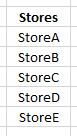
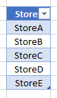
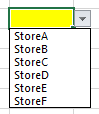
The first step in learning how to create a drop-down list in Excel is to first identify your list of selections. This seems like an obvious step but sometimes people don’t actually set aside a space on their spreadsheet for a list of items and simply hardcode the selections later on. By listing the items, you can easily modify them later and visually see what are the user’s options. In this example, I’m going to give a user a list of stores to choose from:
2. Convert the list into a table
You don’t need to do this but there’s an important reason to do so: if you add items later, the range you select for your drop-down list will automatically update. If you just select a regular range, you’ll have to modify it if you add more options to it later. The goal is to make this as easy as possible. And if you always have to adjust the range for subsequent additions, it’s an easy step to miss.
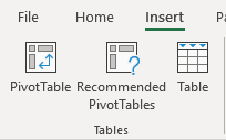
To create a table, just select your range and on the Insert tab, click on the Table button:
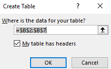
Make sure to include your header in the select and that you tick off that your data includes headers:
Now you’ll likely see some automatic formatting applied to your list that shows it’s now a table:
3. Create a named range
Within the table, where you selections are, create a named range. Just select the cells you want to use (they should be everything in the column) and just assign a name to them. Here’s how you can create named ranges in Excel. Don’t worry if after assigning a named range it doesn’t reflect the name in the reference in the Name Box. Since it’s a table, it’ll still reference the table name. In my example, I created a named range called Stores.
By referencing named ranges, you avoid having to rely on cell references and it’ll make your list dynamic. This is also going to play an important role if you want to have multiple lists, with one based on a prior list’s selections.
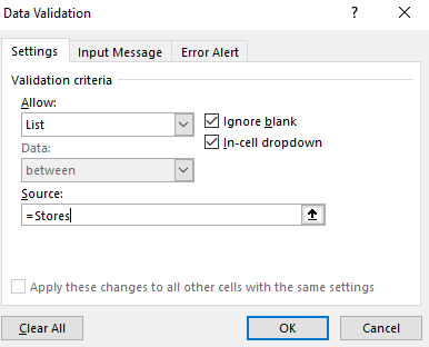
4. Create the drop-down list using data validation
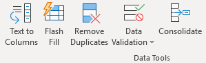
Decide where you want your drop-down list will go. Sometimes it’s helpful to highlight it so that it’s easy to distinguish it from other cells. In my example, I’ve highlighted the cell in yellow. Then, click on Data Validation under the Data tab:
From there, select a List for your range. The list should be equal to your named range or the range of cells you want to use for your drop-down selections. I’m going to set this equal to the Stores named range. When using named ranges, always put the equals sign in front:
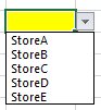
Now, the drop-down list is ready to go:
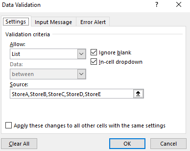
You don’t have to use a named range for a list. You can just select the range manually or you can just type the options in:
As you can imagine, this is a very cumbersome approach and can be very time consuming if you have a long list. Unless you’ve got only a few options that will never change (e.g. yes/no), it probably doesn’t make sense to manually enter the selections this way.
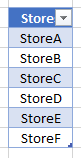
A key benefit of using a named range, within a table, is that if you add selections they’re automatically updated. I’m going to add StoreF to my list of stores. And all that involves is just typing that store directly below the last value in the table:
If I go back to my drop-down list, the selection’s already there:
Had I manually entered the drop-down selections, the list wouldn’t update automatically. I would need to adjust it manually. This can obviously save a lot of time if your list will grow over time.
Creating drop-down lists based on prior drop-down list selections
If you’ve got multiple drop-down lists and want to make them dependent on prior selections, this section is for you. The good news is that it’s largely the same approach. If you know how to create a drop-down list in Excel, adding dependent lists won’t be much more difficult.
You can make some very complicated and nested drop-down lists possible by using a combination of tables and named ranges. In my example, suppose not every store sells the same product. So a scenario can be that a customer is placing an order and selects a store and then in their next selection they can select from a product that’s available in that specific store.
What we’ll need to do in that case is create another named range for that specific store. That range will show the products that store has available. Now, unless the number of selections will remain the same (e.g. same number of stores as there are products available in that store) — which I’m going to guess is unlikely — you’ll want to create a separate table. In this example, I’ll create a list of products just for StoreA, and convert it into a table:
I also need to select the list of products and assign a named range to them. For the named range, it’s important that I assign it the name of the store: StoreA. The reason this is important is that this becomes key to my formula in order to link the previous drop-down selection (where I chose a store) to the new named range.
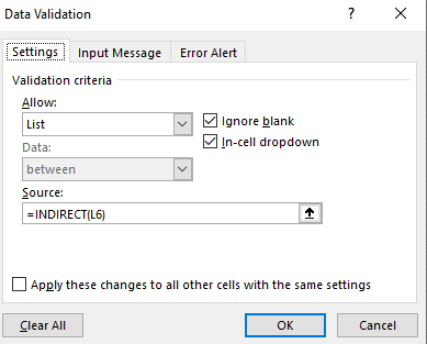
In the next data validation list, I’ll need to use the INDIRECT function and refer to the previous selection (for stores). In my spreadsheet, the cell that contained the store selection was L6, and so my INDIRECT function will need to reference that in the data validation:
Since the range is hardcoded in the data validation settings, if you move your drop-down box you’ll need to update the indirect formulas. Here’s how my second drop-down selection looks now:
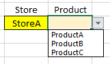
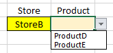
By using the INDIRECT function, the drop-down selections for the product category were updated based on the StoreA selection. I’ll create another table for StoreB where only ProductD and ProductE will be available. Now, when I go to select StoreB, these are what my selections look like:
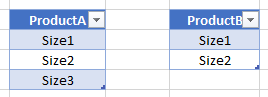
The named range is set to StoreB for those selections. What we can do is drill down even further. Suppose ProductA and ProductB came in various sizes – for simplicity’s sake, I’ll just call them Size1, Size2, and Size3. To do that, I’ll again need to create a table for those selections, and a named range that refers to the product name:
These ranges are called ProductA and ProductB. I’ve put them in separate tables because since there are a different number of options, I don’t want them to be part of the same table. If they were in one table then ProductB would include blanks. And if only selected the first two selections then it wouldn’t automatically update if I added more selections.
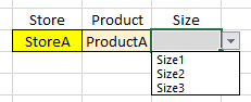
Here’s what my new drop-down selection now looks like if I select ProductA:
For the third drop-down selection, I have to again use data validation and use the INDIRECT function and refer to the adjacent cell. If I select ProductB, I only have two sizes to choose from. Here’s how the drop-down lists look in action:
If you liked this post on how to create a drop-down list in Excel, please give this site a like on Facebook and also be sure to check out some of the many templates that we have available for download. You can also follow us on Twitter and YouTube.