howtoexcel, Author at HowtoExcel.net

Time Off Tracker Template

March 20, 2020

by howtoexcel with One Comment accounting calendar template vacation

If you need to track employee sick days and vacation, then the time off tracker template can help you. This template can also help you decide whether to approve or deny time-off requests as well. Below, I’ll go over the main features of the template and how it works.

Get the Full Version

Setting up the time off tracker

On the Summary tab, you’ll start with a list of all the employees you want to track. This will include their hourly wage, start date, their beginning balance for their vacation days, as well as their vacation rate. The time off tracker template will also track sick days as well.

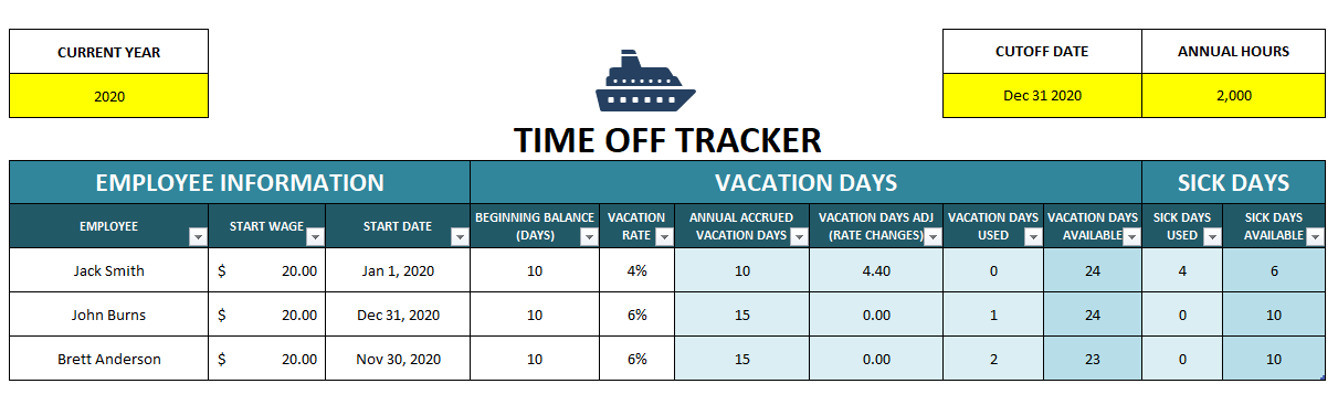
You can enter the current year and the cutoff date if you want to see up to a certain point in time. The annual hours and vacation rate percentage will impact the annual vacation day accrual. Annual hours you’ll probably want to set to either 2,000 (50 weeks x 40 hours) or 2,080 (52 weeks x 40 hours).

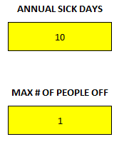
For sick days, there is a section off to the right on the summary page where you can enter the number of sick days people are entitled to annually. You can also specify a maximum number of people that can be off at any one time. This is related to approving requests which I’ll cover further down.

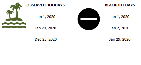
You’ll also see a section for holidays and blackout days for when you don’t want people taking time off. These lists can be as long as you like.

Entering and requesting time off

Whether you want to check if a person can book time off during a certain period or if you want to actually book it, you’ll do this through the Request.Form tab. Here, you can select the employee, the type of request (vacation or sick), and how long they will be off for. This template assumes employees do not work weekends. If the request includes a weekend, it will automatically account for that. Here’s a sample request for someone looking to take Jan. 24 – Jan. 31 off.

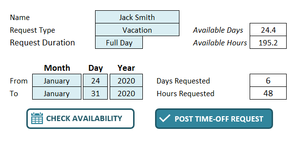
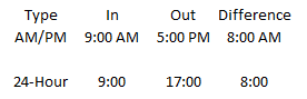
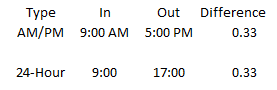
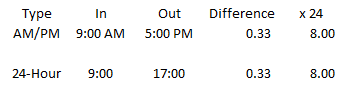
The available days, hours, days requested and hours requested will all automatically fill in once you enter all your selections. You’ll notice the days requested equals six, which isn’t counting Saturday and Sunday. It also assumes these are full days off and hence multiplies the days off by an eight-hour workday to get to 48 hours requested off.

If you want to see if this request complies with your policy (blackout rules, maximum people off) you can click on the Check Availability button. Then you will see the following summary:

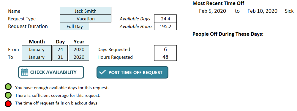
The lights come up green for having sufficient time available and there being enough coverage. But it comes up red because the request includes a blackout day. Over on the right-hand side, you’ll see the person’s most recent time-off requests. It will also show any people who are off during this time.

You can still proceed and click the Post Time-Off Request button either way. It will post the information into the Timeoff tab:

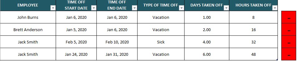
If I double-click on any of the red boxes to the right, it will delete an entry. There is no data that needs to be entered on this tab, this is simply for record-keeping. The Timeoff tab is used to populate other areas of the spreadsheet.

If I were to go back and try and book another entry on Jan. 31 for a different employee, it will now tell me that someone is off during this time:

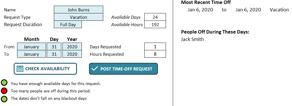
Note: you won’t be prevented from posting vacation if a person already has vacation booked for the same date. But if you make a mistake you can clear the duplicate entry from the Timeoff tab. You can also visually see who is off during a given period on the Calendar tab:

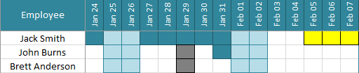
Blackout days are highlighted in black, vacation is dark blue, weekends are light blue and sick days are in yellow. In the above example it shows the one employee who took a vacation day during the blackout period. The color code for vacation overrides the blackout formatting. From this, you can also see that two employees were off on Jan. 31.

Entering in partial-day requests

If an employee is taking a half-day or only a certain amount of hours off rather than a full day, you can select the Partial Day option from the drop-down in the Request.Form tab. A new field will appear, allowing you to enter the hours per day:

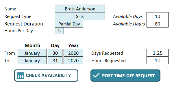
In this example, this employee is requesting 5 hours off on both Jan. 30 and Jan. 31. The employee is requesting a total of 10 hours off, or 1.25 days. If you need to do a partial request, you can’t mix and match with full-day requests, you’ll need to do them separately. Even if the hours are different, multiple requests will be needed.

Whether an employee takes a full or a partial day off, it’ll look the same on the Calendar tab.

Adjusting for rate changes

One of the more complex calculations this time off tracker template factors in is if an employee moves to new pay rate or if their vacation rate changes during the year. This is where the Ratechanges tab comes into play. You select the employee, the date that the change is effective as well as the date it ends – this can be left blank if there’s no further rate change. The purpose of the end date is if there are multiple changes for an employee during the year.

Then, you enter the new hourly wage and vacation rate. Enter both numbers. For instance, if an employee now accrues 6% vacation rather than 4%, you’ll want to enter the new vacation rate but you’ll also want to enter in their hourly wage as well, even if it remains the same. This is important so that the formula calculates correctly.

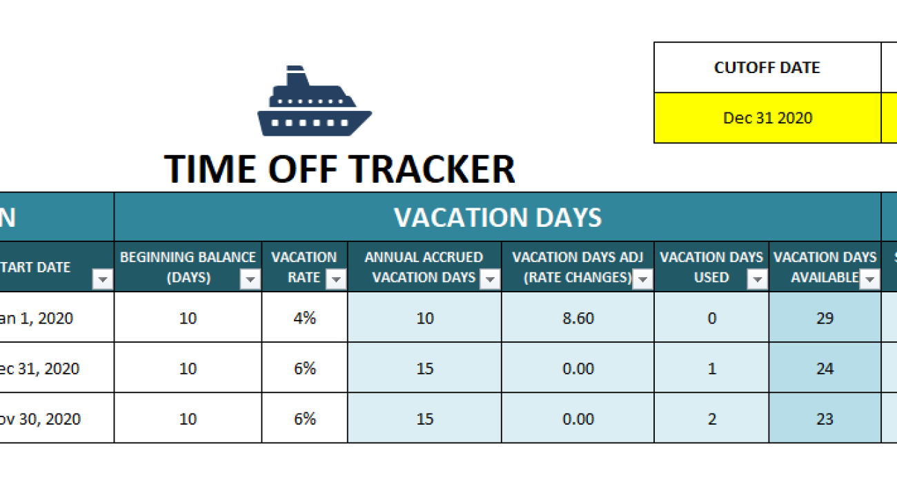
This calculation will spit out a change in daily accrual as well as a total adjustment for the year based on the cut-off date. This adjustment will populate on the Summary tab under the Vacation Days Adj (Rate Changes) field.

As with any complex calculations, always be sure to double-check these numbers against your own. Especially when it comes to multiple rate changes a year, it’s important to ensure the data is entered correctly and that the correct number of days are being accrued. Although I’ve tested the spreadsheet, it’s impossible to factor in every possible situation and so I cannot guarantee 100% accuracy in all situations.

If you’d like to test out the template, you can download the free version here which is limited to tracking five employees. The full version has no limits and there are no ads and the code is fully unlocked:

Get the Full Version

If you liked this post on the time off tracker template, please give this site a like on Facebook and also be sure to check out some of the many templates that we have available for download. You can also follow us on Twitter and YouTube.

How to Lock Cells in Excel

March 14, 2020

by howtoexcel with No Comment formatting intermediate ranges security

One of the most frustrating things that can happen to the spreadsheet you’ve spent hours or days on is when someone overrides a formula or a cell with important information. That why it’s important for people making and designing spreadsheets to be familiar with how to lock cells in Excel. It’s not a difficult thing to do and it can save you a lot of headaches down the road. There are two ways you can go about doing it. I’ll start with the approach that should work even on older versions of Excel:

Step 1: Unlock all the cells

By default, Excel sets that status of every cell to locked. However, until you actually protect a sheet none of that goes into effect. But you’ll actually want to undo that. The first thing you should do is select all the cells (CTRL+A) in your sheet and then go into Format Cells (CTRL+1). From there, go into the Protection tab where you’ll see this:

The protect cells tab on the format cells option.

Untick the ‘Locked’ box and this will leave all the cells unlocked. It sounds like the opposite of what you want to do. However, it’s easier to unlock everything and then re-lock the cells you really need locked. Doing the reverse is going to be more time-consuming.

Step 2: Select the cells you want to protect and then lock them

Now, its time to select the cells that you want to lock. Formulas, any sort of rate schedules or information that shouldn’t be changed are things you’ll want to identify. Once you’ve selected them all, you can go back into Format Cells and this time you can re-check the box to have them locked. If any of these cells contain formulas that you don’t want people to see, you can also tick off the Hidden box. Doing this will prevent anything from showing up in the formula bar when someone looks at one of these cells.

Step 3: Lock your worksheet

Even though you’ve already selected which cells you want to be protected, nothing’s technically happened just yet. What you still have to do is lock the worksheet itself. On the Review tab, you’ll have a button to Protect Sheet. Click on that, and you’ll have the following options to choose from:

First thing’s first, you’ll want to put a password in. Otherwise, there’s really no point in protecting these cells if someone can just unlock the sheet without any password.

By default, Excel selects the first to options when protecting cells, allowing users to select both locked and unlocked cells. However, you can untick the locked cells if you don’t want them to be able to even select locked cells. If your goal is just to protect cells, these two options should suffice. But you can also restrict formatting cells, inserting and deleting rows as well.

Once you click OK, if you’ve entered a password, you’ll be prompted to re-enter it again to confirm it. Now your cells are protected. If you attempt to change the value on any of them you’ll get the following error message:

Error message in Excel when trying to change the value of a locked cell.

If you want to be able to change those cells, you’ll now have to go back to the Review tab and click on Unprotect Sheet. There, you’ll be asked for a password if you’ve entered one.

Optional step: highlight the cells you plan to lock

To prevent frustrating your users, you may want to take an additional step and highlight the cells that they either should or shouldn’t enter values in. This will avoid them getting frustrated with error messages popping up when they try and make changes. Highlight cells can make it a lot easier for users to identify which cells they should edit.

Tip: here’s a quick way to to find all your formulas

If you don’t want to hunt down all the formulas in your sheet that you want to protect, the good news is it’s easy to find them. You can use CTRL+~ to toggle showing formulas or values on your worksheet. However, there’s an even easier way to select all your formulas. By pressing F5 you’ll get the Go To box:

Click on Special (this is greyed out once you’ve locked the worksheet, so you’ll want to do this beforehand). Then, click on Formulas in the next menu:

Selecting formulas in the Go To Special box.

Click OK and now all your formulas will be selected. From here, you can go to the Format Cells options and make sure they’re locked or hidden.

What if you’ve made a mistake and protected the wrong cells?

If you need to make a correction to which cells you’ve selected, all you need to do is to unprotect the sheet. Then repeat steps 1-3. But you may notice something odd when you go back to unlock all the cells:

Protected cells showing a mix of unlocked and locked cells as well as hidden and unhidden.

This is how the checkboxes will show up if not all cells are locked and not all cells are hidden. You’ll only see the boxes blank or ticked off if all the cells have the same values (e.g. protected or hidden). Clicking once on each of these text boxes will turn them into checkmarks:

All selected cells are hidden and locked.

If you were to click OK then all the cells would be locked and hidden. Clicking these checkboxes an additional time will make them all unlocked and unhidden (but not until you protect the worksheet):

All the cells are set to be unhidden and unlocked.

The alternative approach: Protect cells in Excel using the Allow Edit Ranges option

Below, I’ll show you another way how to lock cells in Excel that doesn’t require unlocking and re-locking cells. Rather than following steps 1-3 what you can first do is use the Allow Edit Ranges button on the Review tab. Pressing that button will give you the following options:

From here, you can click on the New button. Next, select a range that you want users to enter data on:

Creating a new range that users can edit.

In this example, I’ve set a name of Range1 to everything in column A. I’ve also put no password for this range. Now, if I go to protect my entire worksheet, I can still edit any cell in column A (regardless of it is set to locked or not). If I had added a password for that range, I’d be prompted to enter it before gaining access to the range:

You also have the option to designate certain users who don’t need a password to edit the range. You can do this by clicking on the Permissions button:

Changing the permissions of who doesn't need a password to access a specific range.

What’s also convenient about the Allow Edit Ranges feature is that you also can protect the sheet right from its options.

Which method should you use?

Ultimately, both methods can help you protect your cells and formulas in Excel. If your worksheet is very structured and there are only certain places where users should make changes, then using the Allow Edit Ranges approach probably makes a lot more sense.

If, however, most of your cells should be editable and there are only a few cells that you need to lock or they’re spread out all over the place, then the first method may be preferable.

Either approach can work and it may just come down to your personal preference on how to lock cells in Excel.

Adding additional controls—locking down the workbook

If you want to take things a bit further and prevent people from modifying, viewing, or deleting worksheets, what you can do is protect your workbook as well. This is a simpler than how to lock cells in Excel and all that you need do here is just click on the Protect Workbook button and put a password on your entire workbook. Doing this will prevent users from renaming, moving, deleting, or hiding worksheets.

If you’d just prefer users don’t see certain worksheets and don’t even see that they’re there, you may want to consider using VBA to hide them without having to lock your entire workbook down. In some cases, locking a workbook may work well at preventing worksheet changes, but it’s an all-or-nothing approach: you can’t pick and choose which worksheets they can change — that’s where VBA can help.

If you liked this post on how to how to lock cells in Excel, please give this site a like on Facebook and also be sure to check out some of the many templates that we have available for download. You can also follow us on Twitter and YouTube.

How to Do a Weekly Sales Analysis and Compare the Same Days of the Week

March 7, 2020

by howtoexcel with No Comment accounting dates forecasting intermediate

Whether you’re doing a forecast or looking back at how your sales were over a period of time, it’s important to ensure that you’re comparing apples to apples. While monthly and yearly numbers won’t have too much noise, once you’re trying to do a daily or weekly sales analysis, that’s when things can get a little challenging.

Below, I’ll show you how you can do a weekly sales analysis where you’re comparing the same days of the week against one another. This will give you an accurate picture of your year-over-year performance.

Step one: determine which day of the week you want to start on

This is a simple step and you’re probably going to go with either Sunday or Monday. But it’s an important one to consider because when you’re looking at weekly sales numbers, you want to be consistent. And while you can refer to the week number when comparing one week to a previous year, saying week 32 is not going to be as useful as saying the week starting August 5 or ending August 11.

In my example, I’m going to use Monday as my starting point to ensure that I’m not breaking up the weekend (the default in Excel is Sunday). To make it easy to compare a week, it will be helpful to create a header for the days of the week so it looks like a calendar.

Step two: entering the first date of the weekday you selected

The first Monday of 2020, wasn’t until Jan. 6 this year, which would be the second week of the year if we start on Mondays. The previous Monday was Dec. 30, which was technically week 53. Weeks 1 and 53 are often abbreviated. For now, just accept that there’s no Monday in Week 1 of 2020. I’ll show you how we can get around this problem further down.

For now, Jan. 6 will be our starting point which we’ll call Week 2. Now, that we have our starting point, we can build out what our subsequent weeks will look like.

For example, if I want to find out the start date for week 40, what I can do is simply use the following formula:

First, I multiply 7 by the difference in weeks. Then, add that to the first Monday value. In this example, it tells me the 40th Monday of the year is Sep 28, 2020. That’s why setting up the first Monday values is important to ensure that it’s easy to get the remaining dates.

This is the easier approach to take. However, later on I’ll show you a way where you don’t have to enter in the first Monday of the year.

Step three: filling in the remaining dates of the week for your sales analysis

Getting the starting date of the week is the toughest part. From there, all you have to add is just add 1 to each subsequent day:

Just adding 1 to the previous date will increment to the next day. No special formulas needed here.

Step four: getting the prior-year date

To get the previous year’s data you can follow the same approach as in step two. However, I’ll use this as an opportunity to show you another way that you can get the data. One that won’t require you to pull out the calendar.

First, we need to know what day of the week Jan. 1, 2019 fell on. To do this, we can just use the following formula:

=WEEKDAY(“Jan 1, 2019”,2)

The reason I put the number 2 as the second argument is because my week is starting on a Monday. If I set it to 1 or left it blank, the default would be Sunday. This is important because if Monday is my first day of the week then it’s day value is 1 and Sunday is 7. Had I used Sunday, then Sunday would have a value of 1 and Monday would be 2. This is why it’s important to know which day of the week you want your week to start on.

In 2019, Jan. 1 fell on a Tuesday, and the formula above gave me the result of 2. (Monday is 1, so Tuesday would be 2). The reason I need to know the weekday is because I need to adjust the date to find out when that week actually started. I use the following formula to do that:

=DATEVALUE(“Jan 1, 2019”)-(WEEKDAY(DATEVALUE(“Jan 1, 2019”),2)-1)

What this formula does is subtracts Jan 1, 2019 from the number of days it is above day 1. It then moves the date back. I can simplify this formula by entering Jan 1. 2019 in cell A1. Then my formula looks like this:

=A1-(WEEKDAY(A1,2)-1))

I no longer need to use the DATEVALUE function and now it’s a bit easier to use. There’s also less chance of an error when entering the date. Now, when I want to find out the first day of the week, I can multiply 7 times the week number and add to this calculation:

=(A1-(WEEKDAY(A1,2)-1))+(7*(B1-1))

B1 is the week number. In this example, if I were to enter Jan 1. 2019 for cell A1, that would give me a result of Dec 31. 2018 for the start of Week 1. Excel also considers this to be the week that contains Week 53 and Week 1. This is where you can get around this issue. By calling this Week 1 of the current year and including December’s days into this week, it will ensure you don’t have the Week 53 problem. It may not look great to call the previous year’s dates part of the new year but it avoids having to manually make adjustments for this period.

Using the updated formula, I can change the Jan. 1 date to reflect 2019 and use week 40 to update my comparables for the weekly sales analysis:

From here, it’s just a matter of now using a SUMIF function on your data to pull the sales for each one of these dates and you’ve got your comparable sales numbers. With 2020 being a leap year, you can see that the dates have moved up two days from the prior year. Without the date adjustment, you could have ended up comparing a Sunday (Oct 4, 2020) against a Friday (Oct 4, 2020).

If you liked this post on how to do a weekly sales analysis, please give this site a like on Facebook and also be sure to check out some of the many templates that we have available for download. You can also follow us on Twitter and YouTube.

How to Remove Time From Excel Date

February 29, 2020

by howtoexcel with No Comment dates find intermediate left mid parse tips & tricks

If your data contains date and time, and you only need the former, there are ways for you to remove time from the excel date. The first step, however, is in determining whether your data is in date format or whether the information is stored as text. Depending on which one it is, it will change how you will need to manipulate the data.

You can use the TYPE function to determine whether your data is in text or numeric format. The function evaluates a value and if it is numeric it will return 1 and if it is text the result will be 2. That will determine which path you need to focus on: converting a text date or just pulling the date values that you need. The latter is the easier of the two approaches.

Removing time from a date value

If the data is in date format, then it’s as easy as using the DATE function to pull out the fields you need. Let’s start with a date that shows the following:

2020-02-29 12:00:00 PM

It has more detail than we need with the time in there but it also has everything that’s needed—year, month, and day. The easiest way to pull out the date is using a formula as follows (where A1 is where the original data is):

=DATE(YEAR(A1),MONTH(A1),DAY(A1))

The DATE function takes three arguments: year, month, and day. By pulling these values out from the cell that has the time, we’re effectively creating a new value that has everything except the time. Now, if you don’t want this to remain a formula what you can do is copy the cell with the date and not the time, and paste it as values. Now, you’re left with hard-coded date values that do not contain the time.

As mentioned, this is the easy part of the process. The more difficult one is if your date is stored as text and where the DATE function results in an error if you try the above calculation. Let’s take a look at how to remove time from an Excel date when it’s in text format.

How to extract the date from a text field

If the same value above was stored as text, the formula involving the DATE function would result in an error. To pull the values that are needed to arrive at a proper date value, we’ll need to parse the data. Parsing can be a bit complicated but when you’re dealing with text, it’s the only way around getting the data you need.

In the above example, the date fields were separated by hyphens but it could be that slashes are used as well. Ultimately, it doesn’t matter, so long as there is some pattern that separates the month, day, and year fields. We will still use the DATE function. But in order to put the correct values in, pulling out the key information is going to be the challenging part.

Let’s start with pulling out the month, since in a month-day-year format, it’ll be the first value and thus, the easiest to extract. Here’s how the formula to pull the month would look, again, assuming A1 is where the data is:

=LEFT(A1,FIND(“-“,A1,1)-1)

Since the month is the first value, we use the LEFT function to pull the characters at the beginning of the cell. A1 is the cell we’re looking at, and the second argument is the length of the string to pull. Here, we’re looking for the dash(-) within the cell and subtracting one character so that the dash itself isn’t included in the extraction. This formula would produce a value of ’02’ and correctly return the month value.

To get the day is a bit trickier since it’s between dashes. It’s still possible to extract it but the formula is a bit more complex and requires using the MID function. Here’s the function with just the first two arguments filled in:

=MID(A1,FIND(“-“, A1 )+1,

The first part of the formula specifies the starting point. For here, we’re again using cell A1 but this time we’re looking for the dash using the FIND function to indicate where the second value begins. We add one to this value to ensure that we aren’t starting at the dash. Here’s what the next argument looks like, for the length of the value:

=FIND(“-“,A1,FIND(“-“, A1,1)+1)-FIND(“-“, A1,1)-1)

Here what we’re doing is using the FIND function to search for the dash but this time we aren’t starting from the first position but are starting from where the first dash was found, and adding a one to that. Then we subtract where the first dash was found, and the difference is the length of the string. It’s a complicated, nested function but it does what we need it to do. The completed formula for the day looks as follows:

=MID(A1,FIND(“-“,A1,1)+1,FIND(“-“,A1,FIND(“-“,A1,1)+1)-FIND(“-“,A1,1)-1))

The last part is to extract the year. And because this comes after the second dash, we’re going to need to nest two FIND functions, not just one. You could try and always start from a certain number, for example, the seventh character if your date format will always by mm-dd-yyyy. However, using the FIND function ensures you aren’t taking any assumptions (e.g. they may be leading spaces). I also avoid hardcoding numbers in formulas whenever possible. Here is the formula that remains for the year function:

=MID(A1,FIND(“-“,A1,FIND(“-“,A1,FIND(“-“,A1,1)+1))+1,4)

The nested FIND functions are needed to ensure that I’m starting to search for the dash after the second instance was found. I use the number four for the last argument because rather than making this formula even more complicated, I figure the year will either be two characters or four, and it won’t deviate. If your data contains two characters for the year, then you can just change the final argument accordingly.

That leaves us with this long formula to extract the date for the mm-dd-yyyy:

=DATE(MID(A1,FIND(“-“,A1,FIND(“-“,A1,FIND(“-“,A1,1)+1))+1,4),LEFT(A1,FIND(“-“,A1,1)-1),MID(A1,FIND(“-“,A1,1)+1,FIND(“-“,A1,FIND(“-“,A1,1)+1)-FIND(“-“,A1,1)-1))

It’s a complicated one so it may be easier to just copy and paste it rather than trying to reconstruct it yourself. If your original date is in dd-mm-yyyy format, here is a formula for that:

=DATE(MID(A1,FIND(“-“,A1,FIND(“-“,A1,FIND(“-“,A1,1)+1))+1,4),MID(A1,FIND(“-“,A1,1)+1,FIND(“-“,A1,FIND(“-“,A1,1)+1)-FIND(“-“,A1,1)-1),LEFT(A1,FIND(“-“,A1,1)-1))

This just involves flpping around the formulas to grab the month and day. If your dates use “/” instead of “-“, then you can just to a find and replace in the formulas above to replace all the “-” with “/” or whatever else your system may use. Regardless how the data is separated, you can adapt the formula to how your data looks.

As you can see, having your data in the right format can make this process a whole lot easier. It’s once you get into text that it becomes much more challenging in pulling the date out. And again, once you’ve got the data you want, copying and pasting as values will ensure you don’t have to keep both the old and new data together.

If you liked this post on how to remove time from Excel date, please give this site a like on Facebook and also be sure to check out some of the many templates that we have available for download. You can also follow us on Twitter and YouTube.

Bank Reconciliation Template With Side-by-Side Matching and Automatic Matches

February 23, 2020

by howtoexcel with One Comment accounting bank reconciliation macros template

UPDATED VERSION: Check out the new 2023 version of this bank reconciliation template

This bank reconciliation template is an update from an earlier file that was made three years ago. It offers many of the same features with some notable improvements, and I’ll go over both in this post. I’ll start off by highlighting the key features and how it can help improve the bank reconciliation process for you.

Matching transactions is easier than ever in this new bank reconciliation template

In the earlier version, the bank reconciliation template looked at the total of transactions for a day or that matched criteria and so it didn’t make match individual items. It can be a mixed bag since some people prefer one way of matching (e.g. multiple cash transactions on a book entry matching up to one large bank deposit amount versus having one deposit for each entry). This template tries to make both methods a bit easier.

The auto-matching feature takes care of the latter approach where each line is effectively given a unique id that will be used to match against other transactions. This is ideal for one-to-one matches where you don’t want to look at just the totals.

If you’ve used the earlier version of this file, you’ll know that in this template, you can set up categories and keys associated with them. For example, if a check transaction shows up on your accounting system as CK#1234 you can create a rule in this template to say anything with CK in the description is categorized as a check and that the numbers that follow the number sign form the key, or the unique identifier. You can create these rules in the Setup tab.

Here are a couple of examples as to how this looks:

setting up categories and keys on the bank reconciliation template

The Category is just the name of the category and the Identifier is what Excel will be looking for in the item description to see if it falls into that category or not. For checks, I’ve used the use numbers after identifier to say that what comes after CK# is what should be the key or the criteria that the template will be looking for when auto-matching. If there is no criteria, you can leave this blank and it’ll simply look at the amount and the category. However, this can be less accurate depending on if you have duplicates and similar data in your bank and book downloads.

You can also cap the length of the key, which is what I did in the above example, setting the Length of Key to 4. What this does is say that only the first four numbers will be pulled after the identifier. You can leave this blank and everything will be included. There is also a section for Gap if you don’t want it to immediately start pulling numbers after it finds the key. For instance, if I used CK as the identifier rather than CK#, then I’d want to set the Gap field to 1, to ensure that it skips over the next character, which in this case would be the # sign. But if you want to immediately pull data after the identifier, you can leave the Gap blank.

Alternatively, you can also just use the date as your key but that will not be very precise. The template and auto-matching will only be as strong as the rules that you put into place.

Manually matching transaction is easy, too

Even if you can’t auto-match all your transactions, I’ve tried to make this template as easy as possible to bulk match transactions as well. While the auto-matching is designed to help one-to-one matches, it’s also possible to match multiple transactions to one. This can be done using the Reconciler, which can be accessed via the Ribbon:

Ribbon buttons on the bank reconciliation file.

In the previous version, these buttons were within the file. Now, they’re on the home tab within the Ribbon, making it easy to access from anywhere in the file. Select a transaction from either the Book or Bank tabs and click the Reconciler button and you’ll have an interface where you can easily match transactions side-by-side:

In the previous version, side-by-side matching was not possible in the Reconciler and this allows you to easily do your matching within this interface. If I select the first transaction, which is a wire transfer, it will show me all the possible wire transfers I can match it to:

However, the ability to match the transactions won’t appear until I have the credits and debits matching an equal amount on both sides, to prevent running into a situation where I’ve matched an unequal amount:

By default, there will be no warning to pop-up when you’re matching transactions. However, if you prefer there to be one, you can change this in the Setup tab where there’s an option to toggle the confirmation from ‘No’ to ‘Yes.’

With it set to off, you can continue going through and matching transactions to ensure that you don’t have to click boxes before moving on to the next item to match. As it’s set up, you can match multiple items to one amount. However, you can’t match multiple-to-multiple and if you want to match multiple to one, then select the one transaction that will be matched to multiple items when launching the Reconciler. In the above screenshot, any transactions on the left-hand-side can be matched to multiple transactions on the right-hand-side, but not vice versa.

However, there is a SWAP button at the top of the form, which is also new, which can allow you to easily switch between the two views.

On both the Book and Bank tabs, there is a column for Manual Override and if you want to match an item manually you just need to enter a value in here. And that’s what the Reconciler does when you’re matching transactions. This is also where the next key feature comes into play: auditing and correcting your matches.

Audit trail from the Reconciler makes it easy to see which transactions are matched to one another

In the transaction that I matched above, it posted this in the Manual Override section:

You’ll notice that it says Previous BOOK Row 6. What this tells me is that the transaction was reconciled on the Previous OS Items tab, which includes transactions carried over from the previous period. It also tells me the row it was on and that it came from the book side. If the entry were to say Current, then it would be from the current transactions and that it would just be from the Book tab rather than the Previous OS Items tab.

If I wanted to undo this match, I could just press delete and clear the data in the Manual Override column. However, if you do this, be sure to clear off the other entry or entries related to it. Otherwise, you can be out of balance if you only cleared out one side of what was matched.

Reconciling the month

Once you’re done with your reconciliation and you want to see a list of your outstanding items, you can click on the Reconcile Month button in the Ribbon. This will spit out the outstanding items and group them by category. This process is similar to how the older version of the file worked.

When you’re finished and ready to start a new month or period, you can click on the New Month button which will clear the Book and Bank tabs and move any outstanding items over to the Previous OS Items tab. You’ll now be able to start a new month or period.

You can also use the Clear Data tab if you just want to remove everything and start completely from scratch

Testing out the file

If you want to give this file a try, please download the bank reconciliation template for free here. You can test out all the functions. There is a limit of just 25 transactions on the Bank and Book tabs. If you want the full version of the product, including with the code unlocked, please visit the product page here.

If you liked this post on the new bank reconciliation template, please give this site a like on Facebook and also be sure to check out some of the many templates that we have available for download. You can also follow us on Twitter and YouTube.

Compounded Annual Growth Rate Calculator

February 19, 2020

by howtoexcel with No Comment calculator investing statistics stocks

If you don’t want to calculate compounded annual growth rate yourself, you can do it quickly and easily with this free calculator:

Calculating Compounded Annual Growth (CAGR)

Percent Change
Number of Years

[WP-Coder id="1"]

8 Ways to Speed Up Data Entry in Excel

February 15, 2020

by howtoexcel with No Comment data entry intermediate shortcuts tips & tricks

Entering data into Excel isn’t much fun, especially if you’ve got a lot of it to enter. The good news is that there are plenty of ways that you can expedite the process so that it’s more efficient and takes less time. Here are eight ways that you can make data entry in Excel a whole lot quicker:

1. Using tab to cycle through your fields

If you’re entering fields across several columns, using the tab button can make it easier to enter data rather than using the arrow keys. And by hitting the TAB button, once you’re at your last column, you can hit the ENTER key and you’ll start from the beginning of the next line. As long as you keep tabbing over, Excel will remember which column you started from when you press ENTER.

Even if you accidentally tab over one or two fields too many, you still don’t have to use the arrow keys. All you have to do is press SHIFT+TAB and you will move in the opposite direction. It has the reverse effect of just pressing the TAB key. Similarly, the ENTER key will bring you down a row while SHIFT+ENTER will move you up a row.

Anytime you can avoid using the mouse or arrow keys, your data entry in Excel can go a lot quicker.

2. Using CTRL+D and CTRL+R to copy data

If you need to copy data from the cell directly above, you can use the CTRL+D shortcut and it will do just that. And if you want to copy data from the left, then you’ll use CTRL+R. This will work the same as if you were to drag the cells. That means that formulas will copy over as well.

3. Use Page Up and Page Down to cycle through tabs

This is another shortcut that can help you quickly jump through different tabs in your workbook. Page Down will cycle through the worksheets to the right, and Page Up will go through the worksheets that are to the left of your active sheet. If you’re entering a lot of data across many tabs, this will help you avoid having to use the mouse to switch tabs.

4. Entering data in multiple worksheets at once

If you have to enter the same data, the same formula, or if you just need to change the formatting so it’s the same across all worksheets, the good news is you don’t have to do one tab at a time. Instead, select all the sheets that you want to make the changes to and then enter the data or make the changes you need to make in any one of them. If the worksheets are all selected, the changes will be applied to all of them.

Multiple tabs selected in an Excel spreadsheet.

In the above screenshot, I’ve selected Sheet1, Sheet2, Sheet3, and Sheet4. The one I’m currently in is Sheet1. Any changes that I make in that sheet will carry over to the others.

Be careful, however, because if you make a change in cell A1, then A1 will change for all the worksheets that you’ve selected. If your data is structured slightly differently in the sheets, this may give you some unexpected results. This should only be used if your data is in the exact same structure. For formatting, however, it’s an easy way to apply formatting to many sheets at once. But when you’re entering data or formulas, you should double-check which cells you’ll be entering the data into to make sure that they’re correct and won’t cause issues across all the different sheets.

5. Moving quickly throughout your worksheets

Tabbing over can be helpful as you’re entering data, but it may not be of much help if you need to go to the end of your data set. For this, there are a couple of things you can do. If you want to go to the last row of your data, double click on the bottom of your active cell, which will send you to the last row where data is entered in that column. If you want to go to the furthest column to the right, double click on the right border of your current cell selection.

Alternatively, what you can do is use the CTRL key along with the arrow keys. For instance, if you want to go to the last row in the column that you’re in, use CTRL + DOWN. And if you want to go to the furthest column in the row that you’re in, use CTRL + RIGHT.

6. Make sure to freeze panes

When you’re entering data into many different columns, freezing the headers at the top can make it easy to ensure you’re entering the right information in the correct field. You may forget where you are if you’re working on many different fields and by freezing panes, you can ensure you have enough data to look at regardless of how many rows down you, and that can lead to wasted time. If you’re not familiar with freezing panes, this post can help give you a quick overview.

7. Maximize your white space

If you’re on a laptop or a small screen or just need to see a lot more data, you can hide some unneeded space in your spreadsheet. That can make it easier to enter data and minimize distractions. For starters, you can minimize the ribbon by double-clicking on any one of the heading names:

You can still use the ribbon and access it, but this way it gets out of your way unless you actually click on any of the headings again. To undo this, just double-click a header and you’ll get your full-sized ribbon back.

Next up, click on the View tab where you’ll see a few more things you can change:

Here you can uncheck the Formula Bar and even the Headings, assuming you don’t need to see this, of course.

Excel spreadsheet with hidden formula, headings and ribbon minimized.

At this rate, your spreadsheet is looking more like just some plain lined paper. And if you need any more white space, then maybe you’re better off simply investing in a bigger monitor or shrinking your resolution.

8. Use a second window

If you have a second monitor, and even if you don’t, you can create a second window within Excel. Whether you’re entering data into multiple different sheets or even if you just want to enter data into multiple areas within the same sheet, a second window can help. This way, you’ll avoid having to jump back and forth. To this, go back to the View tab where you’ll see an option to open a New Window:

Open a new window in Excel using the View tab.

From here, you can move your new window onto another monitor or you can just do a split-screen if you only have one. With Windows 10, you can snap windows to the left or right-side of your monitor, making it easy to see two Excel windows at once.

Got any other tips? Submit yours!

Have any tips of your own that use that improve your data-entry experience in Excel? Feel free to email [email protected] and let us know what you’ve found helpful and if we use it in an updated list, we’ll credit you.

If you liked this post on how to speed up data entry in Excel, please give this site a like on Facebook and also be sure to check out some of the many templates that we have available for download. You can also follow us on Twitter and YouTube.

Why You Shouldn’t Bother With Excel’s New XMATCH Function

February 8, 2020

by howtoexcel with No Comment functions index intermediate match

Last year, Excel released some updates including the unveiling of XLOOKUP as well as XMATCH. In this post, I’ll show you how to use the XMATCH function and also why you may not have a need for it.

For this example, I’m going to use a list of the stocks with the largest market caps on the U.S. exchanges as of Feb.7, 2020. Here’s what my data looks like:

Top stocks listed on the NYSE and NASDAQ as sorted by market cap.

XMATCH can achieve the same results as MATCH does when looking for data, but if you wanted the same functionality you could just use MATCH. Instead, let’s start by looking at some of the other things that Microsoft claims XMATCH can do.

XMATCH is not a suitable COUNTIF replacement

One of the things that XMATCH can supposedly do is when you’re looking up numbers, it will count the number of times that values fall above or below a threshold. For this example, we will look at the number of stocks on this list with market caps of more than $1 trillion.

To do this, you would use $1,000,000,000,000 as your lookup value and set the third argument of the function, called match mode, to 1, which looks at an exact match or the next larger item. Here’s how the formula looks like:

Where L6 is the cell that has the number that XMATCH will search for (1,000,000). This formula correctly gives me five matches that are more than $1 trillion that appear on the list. However, if I include the header, the results change:

This leads me to believe that it’s still looking for the closest match and not really counting the number of values that meet the criteria. And indeed, when I changed some of the market cap numbers so that they were more than $1 trillion, XMATCH didn’t compute them correctly since they weren’t in descending order. I’m assuming what Microsoft is implying with XMATCH is that if your data is sorted in ascending order, it would be able to tell you where the smallest value is that meets your criteria. For example, The sixth row in the data set was $1.02 trillion and that was the lowest entry that was more than $1 trillion. Technically, if the data was in descending order then everything above that will be more than $1 trillion.

However, that’s very different from actually counting the numbers over that threshold. And that’s why COUNTIF is still vastly superior to XMATCH. Here’s how the two functions worked when I added four additional entries (not in order) of more than $1 trillion, bringing my tally to nine:

In the COUNTIF function, it still correctly counted nine instances where there was more than $1 trillion on the list. XMATCH, meanwhile, continued to point to the sixth row.

These issues are confirmed when we look at the number of values below $1 trillion:

The -1 argument in match mode is the opposite of 1, and it looks at the exact match or next smaller item. However, the results, as you can see, were very different and not what I would have expected. It appeared to point me to the closest number to $1 trillion without going over. COUNTIF, meanwhile, continued to correctly count the number of items that were below $1 trillion. And with 1,000 items in my data set, it makes sense that 991 were below if nine were above the threshold. Unfortunately, that same logic doesn’t work with XMATCH.

As a replacement for COUNTIF, XMATCH gets a fail as it’s clear that it’s not really counting the number of instances. Only under very specific circumstances would the function do that, such as if the data was in descending order. And even then, you’d still need to do a calculation for the header or if you’re looking at the number of items below a threshold. It’s more trouble than it’s worth and COUNTIF has the benefit of also being available in older versions of Excel, even going back to Excel 2000. That’s important if you’ll ever need to work on an older version of Excel.

Using XMATCH to search for text is not any better than using MATCH

If you’re using XMATCH for matching text, it won’t be able to count the instances but you can use it to find the first instance of it. Some companies trade under multiple tickers and you’ll notice Google’s parent company Alphabet shows up twice in this list. Here’s what happens when I try to use the XMATCH function to find the first instance:

I’m using a question mark after the text as that’s what Microsoft instructs users to do when looking for partial matches. However, if I ignore that advice and use an asterisk and specify I’m using a wildcard match, then it appears to fix the issue:

You may be wondering how the regular MATCH function did:

Besides changing the last argument, the functions are nearly identical in how they’re used to find partial matches.

Let’s compare how the functions work when we’re looking at exact matches. For this example, I renamed the multiple Alphabet names so that they only spell out Alphabet with no mention of share classes, e.g. so they’re exactly the same. Here’s how XMATCH does on a simple match calculation:

Comparing MATCH to XMATCH on exact matches.

Here again, there’s little distinction between the two functions.

Microsoft also advertises that XMATCH can be used in an INDEX/MATCH combination, but even that seems kind of pointless.

Using XMATCH with INDEX makes little sense

Let’s use these functions to grab the intersect between the company name and its dividend yield. The name is in column B while the dividend yield is in column G. All the headers are in the first row. Here’s how the formula looks like with the use of XMATCH:

In this example, XMATCH correctly pulled the right percentage for Visa’s dividend yield of 0.59%.

That would be really, really cool if the MATCH function didn’t already do the exact same thing. By getting rid of the X in the XMATCH function, thus making it just a MATCH function, and adding a 0 for the third argument, I get the same exact result:

XMATCH doesn’t improve upon anything when it involves the INDEX and MATCH combination. We’re talking a slight change to the syntax, that’s about it. And again, from a functionality point of view, there’s just no reason to swap a new function in when the existing one works just as well, especially since there’s no backwards compatibility on older versions of Excel for XMATCH.

What XMATCH can do well

Everything that the MATCH function can do, XMATCH can do as well. That’s the good news. There is, however, one thing that XMATCH can do better, and that’s look for data in the reverse order. Here’s a simple example of how both functions work when we’re looking for the first value that contains the word Alphabet:

Both functions correctly yield the same results. Again, the change here is mainly to do with syntax. Under the new XMATCH, if I set the third argument (match mode) to 0 and look for an exact match, I’ll get an error. But if I set it to 2, which is wildcard character match, it will produce the correct result: Alphabet, which first shows up on the fifth row. However, it’s easy to see how this will confuse users who are familiar with MATCH and just use 0 for the third argument, which will also produce the correct result in this case. This is another example of where the syntax has gotten more complicated and not given the user any additional advantage.

The one exception to that, however, is if you want to do a search in the reverse order. MATCH currently will go from the first row and work its way down. Once there’s a match, it will stop there. Here’s how the XMATCH function performs when we’re doing a last-to-first search, as indicated in the fourth argument where the value is -1:

This time XMATCH does correctly pull the sixth row, which is where Alphabet would first show up if we were looking from the bottom and moving up. MATCH, unfortunately, doesn’t have the option to do that and a user would have to rearrange their data to get the same result.

The reverse-order search is the only advantage I can see from testing out XMATCH. Unfortunately, the new function doesn’t add anything significantly new and at worse, it can lead to incorrect results, especially if you’re planning to use it to replace COUNTIF.

Why learning new functions may not be worthwhile, at least not initially

It’s possible that in future updates the XMATCH function will work better but for now, there’s not a whole lot of reason to use it. One of the biggest disadvantages of new functions is that they won’t be helpful to you if you’re working on an older file. It’s not uncommon for people to be working on Excel versions that are more than 10 years old. Not everyone needs the latest-and-greatest version, and mastering a new function may not prove to be worthwhile, especially when older functions work just as well, if not better.

If you liked this post on how to use XMATCH, please give this site a like on Facebook and also be sure to check out some of the many templates that we have available for download. You can also follow us on Twitter and YouTube.

How to Hide Zero Values in Excel

February 1, 2020

by howtoexcel with No Comment conditional formatting errors formatting iferror intermediate tips & tricks

If you’ve got a big spreadsheet with lots of numbers to look at, it can sometimes be a bit difficult to look at a large chunk of data. That’s where knowing how to hide zero values in Excel can be helpful in reading and analyzing data in Excel. By not seeing the zero values, you can easily focus your eyes on the more important numbers that may need more analysis.

However, it doesn’t have to be just zero values that you hide. Any number that’s insignificant for your analysis can also be hidden. For instance, you can be analyzing a company’s financial performance and choose to hide any movements that are less than 5%. The same principles apply as you would use to hiding zero values. Below, I’ll show you how you can hide not just zero values but any values that you don’t want showing up in your data while still factoring them into totals and any other calculations. You won’t be deleting anything, just masking the information.

First, let’s take a look at how to hide a potentially even bigger nuisance: errors.

How to hide errors on a spreadsheet

To help illustrate how to hide zeo values in Excel as well as other numbers, I’m going to use some real-world data — Amazon’s most recent annual earnings report, which the company released last month. Here’s the company’s income statement from the past three years:

Amazon's income statement over the past three years in Excel format.

If you’d like to follow along, you can download the data from the SEC. First up, I’ll add a few columns showing the change from 2018 to 2019 and from 2017 to 2019. Here’s how it looks just copying the formulas straight down:

Analyzing Amazon's income statement using Excel with error values showing.

I have divide by zero errors as there are rows that have no data. I could just remove these cells but as with anything in Excel, it’s good to be consistent. Rather than deleting those error values, I can get rid of the errors in one of two ways.

The first is by using an IF statement to say that if the denominator is 0 or blank, to ignore the calculation. The second is just to use an IFERROR statement.

Here’s what my formula looks like for the 2018 to 2019 change:

=C5/D5-1

Where C5 is the 2019 data and D5 the 2018 numbers. I don’t need any parenthesis as order of operations ensures the formula will calculate properly. However, it doesn’t prevent me from getting a divide by zero error. Since the numerator can be blank or zero, what I’ll want to focus on is fixing the denominator in D5. To do this, I can add an IF function that looks at whether the denominator is a number. Here’s what my formula will need to look like to remove that error:

=IF(OR(D5=0,D5=””),””,C5/D5-1)

The formula now checks to see whether D5 is either a zero or blank, and if it is, it returns a blank value. Otherwise, it calculates as normal. Now I can copy this formula down and get rid of the error values.

An alternative way to fix this is by using IFERROR. Introduced in Excel 2007, the function can be an easy way to replace errors on your spreadsheet with another value. In this example, I’m going to use empty quotes (“”). The benefit is obvious: it’s a lot easier to use IFERROR than an IF statement, especially combined with an OR function as well. Here’s what my formula would look like with IFERROR:

=IFERROR(C5/D5-1,””)

It’s a whole lot easier and quicker. I don’t have to worry about the logic and all the reasons why the formula might error out. However, it’s not a perfect solution and here’s why: it will correct errors, but it’s possible they’ll be errors you’re not expecting. For instance, if I copied the data wrong or keyed something over and put text in a field where it should be a number, the IFERROR will correct that and you won’t be able to tell whether it’s blank because it is a divide by error problem or something else. That’s where it can be a little dangerous in using this one-size-fits-all approach to fixing error values. As long as you’re okay with that, it’s a perfectly good approach to fixing the divide by zero errors.

Here’s the data now that it’s been cleared of errors:

Analyzing Amazon's income statement using Excel after error values have been hidden.

That looks a lot better but the problem is that it’s still a lot of percentages to look at and it’s difficult at a glance to see what are the big changes are from the prior year. This is where it’s also important to hide zero values in Excel, as well as low values that aren’t useful for analysis.

How to hide zero values in Excel and other numbers that you don’t want or need to see

In order to hide data, it’s useful to use conditional formatting. If you’re not familiar with how to use conditional formatting, check out this post. Conditional formatting won’t remove or erase any data, which makes it a good solution that will keep all the data and calculations intact.

In the Amazon example, there are some pretty large-moving items in the list. Removing zero values won’t do anything and the threshold needs to be big for it to be helpful in hiding the lower values. Let’s start by removing the percentages that are less than 20%. Here’s the formula that I will use in the conditional formatting to accomplish this:

=AND(F5<0.2,F5>-0.2)

Column F is where the % Change from 2018 values are. I need to use the AND function because if I just look at anything that’s less than 20% this will also capture negative movements that are more than 20%. And for now, I want to keep those. I want to remove anything that’s between -20% and +20%, which is what the above formula will capture. If I was only looking to remove the zero values then the formula would be as simple as F5=0.

The next step is to adjust the formatting so that the cell font is white. Changing the color is an easy way to hide a cell’s value if it’s on a white background. While that data is still there, it won’t be visible:

Analyzing Amazon's income statement using Excel with error values fixed and low values hidden.

It creates a lot more white space, allowing me to see a lot more of the bigger values. The problem that I notice, however, is that there are some low values that are creating big movements in percentage. I can go a step further and create another conditional formatting rule that will also ignore the percent change for any item in 2019 that was less than $1 billion (1,000). This is how that formula will look:

=$C5<1000

I need to freeze column C because the conditional formatting will be used for the other change column as well and I don’t want the reference to move. Now, with this adjustment, it makes a much bigger difference and helps me narrow in on fewer items:

I can see that the significant changes from 2018, besides the totals, were in sales, technology and content, and marketing. However, since the growth rate from 2017 is even higher, I’ll need to adjust those percentages to also ignore anything that’s not at least a 50% improvement. Here’s how that formula will look (note that I’ll only apply it for the % Change from 2017 column):

=AND(G5>-0.5,G5<0.5)

Remember, since I’m analyzing percentages, these figures need to be in decimal point. Otherwise, I would be using whole numbers. With those changes, this is how my data looks:

Now I’ve also got a reasonable amount of items I can focus on for the % Change from 2017 column. In addition to the same items increasing from 2018, I notice that fulfillment costs have also shown a significant increase over two years.

The conditional formatting works great in clearing out numbers that I don’t want to see. However, there’s just one small problem…

Analyzing Amazon's income statement using Excel with hidden values showing on a dark background.

If I change the color to anything that isn’t white, those numbers that I hid become visible again. That leads me to another all-important section:

How to hide values in Excel that are on different background colors

You can create conditional formatting rules to address other background colors but that’s just not practical. If you use lots of colors on your spreadsheet the last thing you want to do is create a rule for every different color and make sure the cells are hidden in the same font color. There’s also a problem if someone changes the color too.

That’s why using font color to hide values in Excel isn’t a good idea. The good news is that there’s a much easier way to hide values that doesn’t involve you having to try and match up the color.

Rather than changing the color, what you should do is use a custom number format. Simply use three semi-colons and that will do the trick:

Choosing a customer number format to hide zero values in Excel.

Without going into the details of the different formats you can use, by using three semi-colons you’re telling Excel that you want no formatting to be used whether the amount is positive or negative. Now, my hidden data remains hidden regardless of the background color:

Analyzing Amazon's income statement using Excel with hidden values no longer showing on a dark background.

Now you don’t have to worry about background colors and can easily hide your data in any context.

If you liked this post on how to hide zero values in Excel as well as other values, please give this site a like on Facebook and also be sure to check out some of the many templates that we have available for download. You can also follow us on Twitter and YouTube.

How to Calculate Time Difference in Excel

January 26, 2020

by howtoexcel with No Comment dates intermediate parse

If you need to keep track of time entries, whether for a timesheet or some other purposes, it’s important you know how to calculate time differences in Excel, and that’s what I’ll show you how to do in this post. If you’re just looking for the difference in dates, including months, days, or years, then refer to this post. But if you need time differences, keep reading.

Entering time correctly

In order for the difference in time to be calculated correctly, it should ideally be entered in the right format to start with. Let’s use the example calculating the hours worked for a regular 9-to-5 shift.

You can use a 24-hour clock or AM/PM to enter time. If you’re using AM/PM, then you’ll want to make sure you enter a space between the time and the AM/PM indicator. For example: 9:00 AM rather than 9:00AM.

If you enter it correctly, then the value you just entered should align to the right. This means that Excel has interpreted it as time. You can also tell because in Excel it will show as 9:00:00 AM in the cell details. Normally, you aren’t going to enter seconds but Excel will track those extra zeroes anyway.

If you were to just enter 9AM then you’ll notice after hitting enter that nothing happens and Excel doesn’t align it to the right side of the cell. This means that what you’ve entered Excel is reading as text.

That is a problem because if you want to calculate the time difference correctly, it’ll get a whole lot more complex and require using IF and MID functions. It’s not impossible (and I’ll show you how to do so later on), but it will make it a lot more complicated.

Calculating the time difference

Now that you’ve made sure that the time entries are entered correctly, it’s time to show you how to calculate time difference in Excel. Here’s how it looks if I just take the end time and subtract the start time:

calculating time difference for am pm and 24-hour time

If you’re using the 24-hour clock then it looks okay. However, the calculations are still reading in the time format and while that may work okay for the 24-hour clock, it’s going to cause an issue for the AM/PM. So let’s change the format using the comma style so it doesn’t read like a date. Then, the data looks as follows:

This might seem even more confusing until you realize what Excel is doing. It’s assigning a value between 0 and 1 for the time of day. The value of 0.33 indicates that the time is one-third of the day, which is what an eight-hour shift would be since 8/24 is the same as 1/3.

However, using 0.33 isn’t going to be too helpful if you need hours to be able to track how much someone should earn for that shift. To solve this, simply multiply the time difference by 24. Then, your time difference looks as follows:

calculating time difference for am pm and 24-hour time and converting into hours.

Now you see the eight hours that you may have first expected to see when calculating the difference between these times. Since it’s now reading as a number, you can multiply this by an hourly rate and arrive at the pay that is owing for the shift.

If you’re not looking for hours and just want the total minutes, then all you need to do is just multiply by a factor of 60 to convert the eight hours into 480 minutes.

Calculating hours worked when someone works the night shift

The above calculations work well if someone is working within the same day, but if someone starts at 9:00 PM and ends at 5:00 AM the next day, it’s not going to calculate properly if you simply take the difference between the numbers. In fact, the number would come out negative:

That’s obviously not what you’ll want. To account for this, you’ll need to add an IF statement into our formula. The IF function should look at whether the end time is earlier than the start time. If it is, you’ll want to add 1 to the calculation. Here’s how the formula for the difference calculation would look like:

adjusting time calculations for overnight shifts.

I include the 24 in the calculation so that I don’t need to use an extra cell to convert the difference into hours. All the formula is doing is looking at if the end time is before the start time, and if it is, add a 1 to the end time before subtracting the start time from it. This method will work whether you’re using a 24-hour clock or the AM/PM format:

This method will work even if someone works a 16-hour shift:

Knowing how to calculate time difference in Excel isn’t difficult, and the key points to remember are as follows:

Ensure the time is entered correctly, and
Multiply the difference between the times by a factor of 24 for hours and another factor of 60 if you only want minutes.

Calculating time difference in Excel when the data is in text

If you need to know how to calculate time difference in Excel and you don’t have the luxury of the data being in the right format, the good news is it’s still possible to do so.

For instance, what if you want to enter the entire start and end times within one cell. In that case, you’re always going to be running into this situation. Suppose someone enters the following value into a cell: 9:00 AM-5:00 PM.

The format would be correct if there weren’t multiple times in that cell, which ensures it will read as text. That’s where you’ll need to use some data manipulation that involves using the MID function.

Let’s start by pulling the start time. For this, we’ll grab the numbers that come before “AM” but because it doesn’t matter whether it’s AM or PM, we’ll search for the letter “M” on its own:

=MID(A1,1,FIND(“M”,A1,1))

Here’s a breakdown of the formula:

Argument 1: A1 is the cell we’re looking at.
Argument 2: Start pulling from the first character.
Argument 3: The length of the text goes up until the letter “M” is found.

The formula will yield a result of 9:00 AM. However, you’ll still need to convert this into a number and you can do this by multiplying the result by 1 or putting it inside the TIMEVALUE formula:

=TIMEVALUE(MID(A1,1,FIND(“M”,A1,1)))

This will now give us a value of 0.375 and it can be used for the calculation. Next up, we’ll calculate the ending time. To do this, we’ll again use the MID function but the key is to start pulling the data after the dash (-) sign:

=MID(A1,FIND(“-“,A1,1)+1,LEN(A1))

This one is a bit more complicated, but let’s look at the different arguments again:

Argument 1: Still looking at cell A1.
Argument 2: Use the FIND function to get to the position where the dash (-) is at and then add a 1 onto that to ensure we’re starting from where the number begins and not the dash (-).
Argument 3: Even though you don’t need the total length of the string, you can use the LEN function to ensure the formula get everything that comes after the dash (-).

Doing this will give us a result of 5:00 PM and by again adding the TIMEVALUE function into it, it will give us a result of 0.7083

=TIMEVALUE(MID(A1,FIND(“-“,A1,1)+1,LEN(A1)))

You can now combine these formulas into one to do the calculation with text:

=TIMEVALUE(MID(A1,FIND(“-“,A1,1)+1,LEN(A1)))-TIMEVALUE(MID(A1,1,FIND(“M”,A1,1)))

This will result in 0.33 for the time difference, which is the correct result. However, with shifts that stretch into the following day, you’ll again run into the issue of how to deal with calculating time. If you don’t have night shifts to worry about, you can stop here.

But if you need to factor them in, then the easiest way to do so is using the AND and IF functions. We’ll want to look at whether the last two characters end in “AM” while also looking at whether “PM” is in the text:

=IF(AND(RIGHT(A1,2)=”AM”,(NOT(ISERROR(FIND(“PM”,A1,1))))),1,0)

Here’s a breakdown of the formula:

The first formula inside the AND function looks at the last two characters in the text to see if they equal “AM”
The second function looks for the characters “PM” anywhere in the cell. If it’s not found it will result in an error, that is why the formula begins with NOT and ISERRROR; you’ll want to add a 1 if it isn’t causing an error and “PM” is found.
If both of the above conditions are met, a value of 1 will be returned. Otherwise it will result in 0. This can now be added to the earlier time calculation formula, added to the end time.

Here’s how the complete formula will look like after adjusting the end time in case there’s a cross over from PM into AM:

=IF(AND(RIGHT(A1,2)=”AM”,(NOT(ISERROR(FIND(“PM”,A1,1))))),1,0)+TIMEVALUE(MID(A1,FIND(“-“,A1,1)+1,LEN(A1)))-TIMEVALUE(MID(A1,1,FIND(“M”,A1,1)))

It’s a messy formula but it is only adding the 1 to the end time if it’s a PM start time and ends in the AM. The only thing left would be to multiply this all by 24 to get the entire shift total in hours:

=24*(IF(AND(RIGHT(A1,2)=”AM”,(NOT(ISERROR(FIND(“PM”,A1,1))))),1,0)+TIMEVALUE(MID(A1,FIND(“-“,A1,1)+1,LEN(A1)))-TIMEVALUE(MID(A1,1,FIND(“M”,A1,1))))

The key thing to note is for this formula to work it’s important to leave a space between AM and PM. For example, if I were to just enter 9:00AM, Excel wouldn’t read that properly and it would result in an error. By leaving a space, it helps with parsing the data out, otherwise the formula would need to be even more complex. If it isn’t in that format, it’s preferable to first clean up the data as opposed to building a very complicated, nested formula using IFs and MIDs.

The above example goes over a few scenarios and obviously you can adjust the MID and other functions as needed based on how your inputs look. Pulling date calculations out from text is possible, it’s just no very pretty.

If you liked this post on how to calculate time difference in Excel, please give this site a like on Facebook and also be sure to check out some of the many templates that we have available for download. You can also follow us on Twitter and YouTube.