A drop-down list is a way you can control a user’s input in Excel, to ensure that they don’t make a mistake when entering in data. It can also serve as a helpful way to make your chart more dynamic. In this post, I’ll show you how that’s possible.
Starting with a regular chart
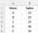
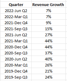
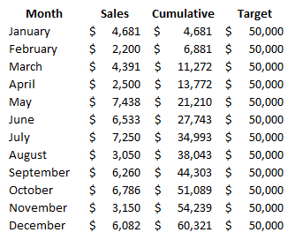
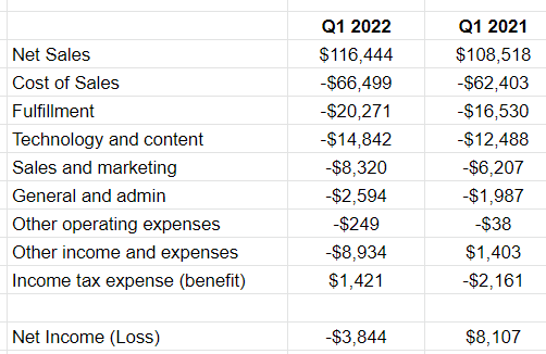
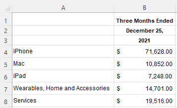
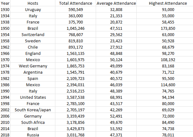
For this example, I’m going to use the following table in Excel that shows historical World Cup attendance between 1930 and 2018. It shows the total, average, and highest attendance at each tournament:
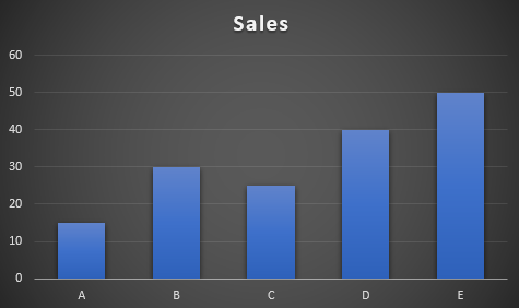
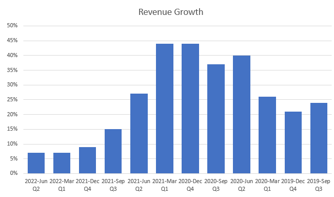
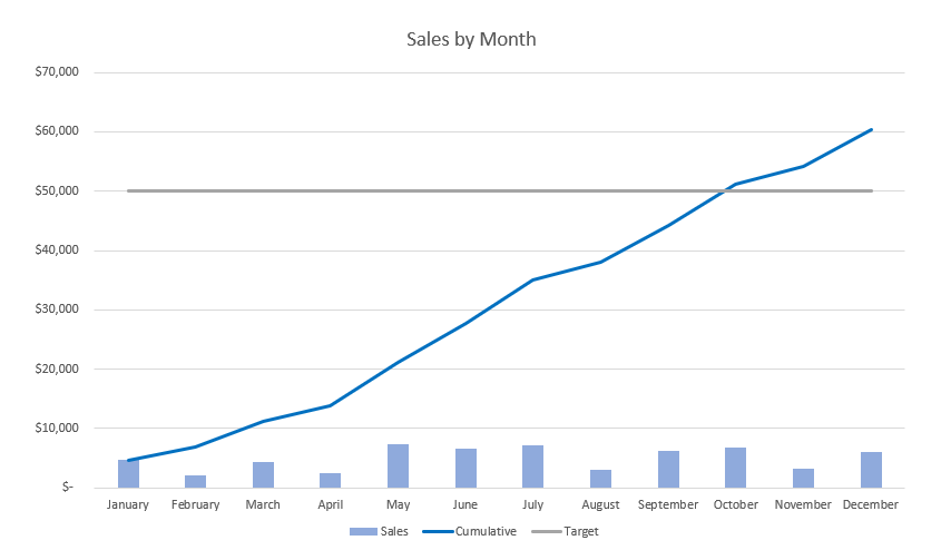
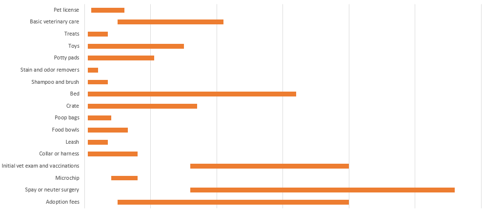
Now, you could chart this out but the problem is that things can get a bit crowded:
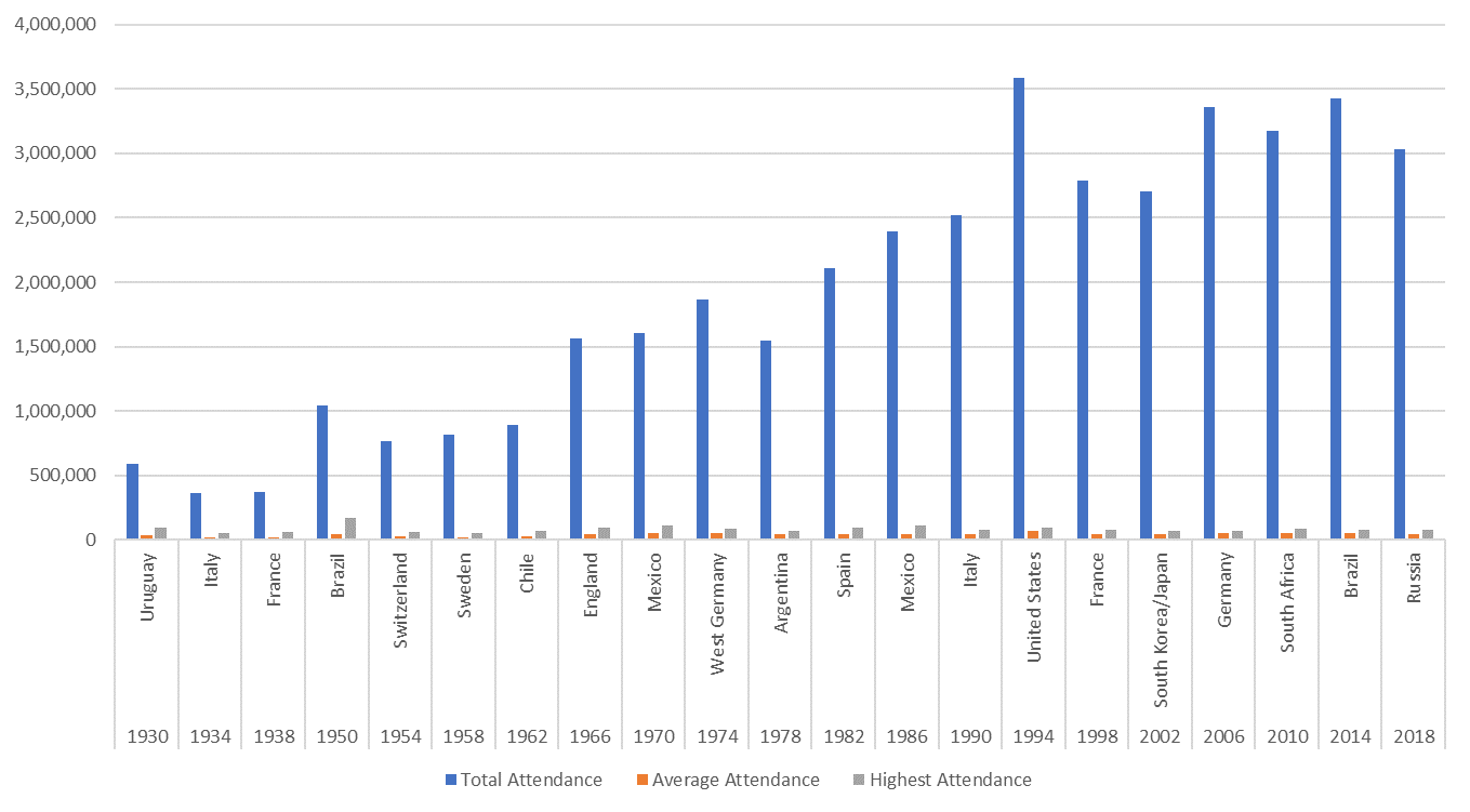
Another issue here is because the chart is looking at total attendance along with average and highest numbers, the scales will distort the chart, making it difficult to compare averages and highest attendances. The solution to this is to use a drop-down list where the user can select which metric they want to see.
Setting up the drop-down list
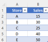
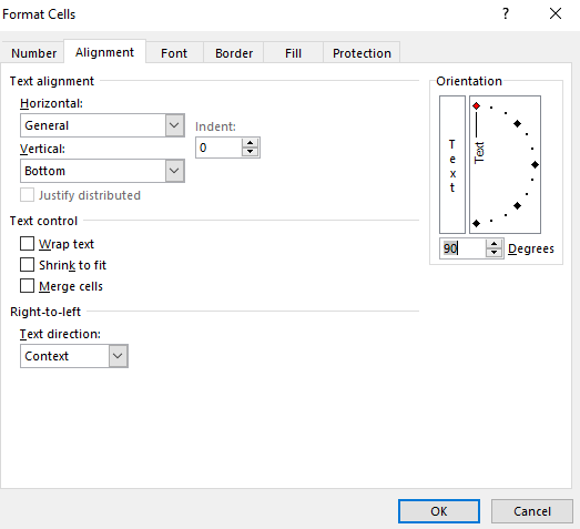
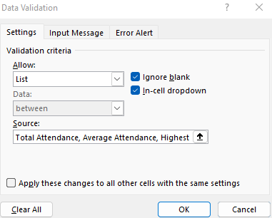
Creating a drop-down list is simple and it involves just going into the Data tab and selecting the Data Validation button, where you can select the List option and enter all the possible selections you want a user to be able to choose from:
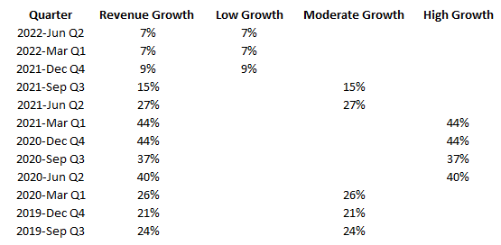
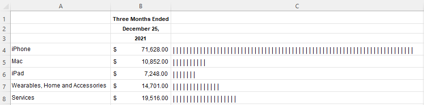
The key is to use the user selection and then populate a column with those values. For example, I’ll set a column header so that it is linked to the drop-down selection. That way, if someone selects Total Attendance, that will be the the header for the new column. I will also use the OFFSET function to determine which of the columns that I’m copying the values over from:
=OFFSET(A2,0,MATCH($F$1,$A$1:$E$1,0)-1)In the above formula, I’m looking for cell F1 (the header that’s referencing the drop-down selection) within the range A1:E1, to see which one of the headers it matches up with. Using the OFFSET function, I can then pluck the value from the correct column. If I copy the formula down, then my new column will be based on the drop-down selection and it will automatically update based on the selection that is made
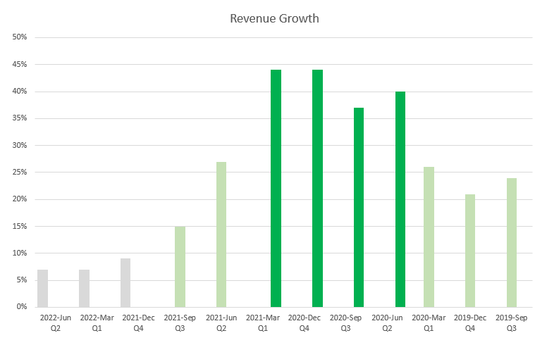
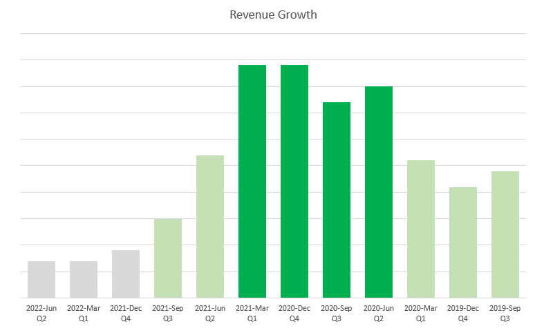
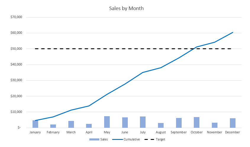
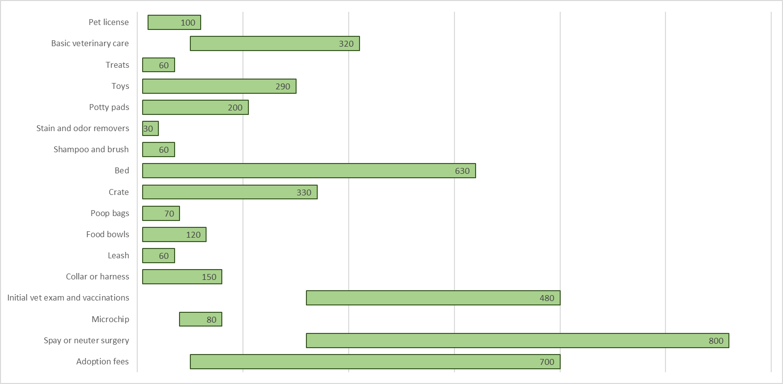
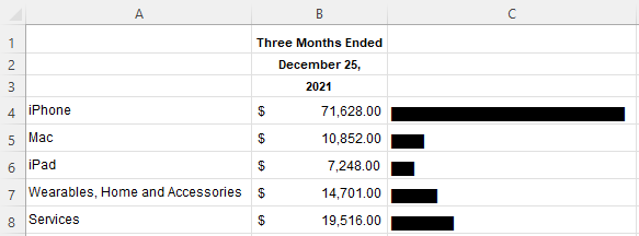
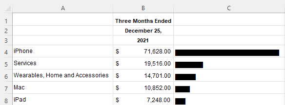
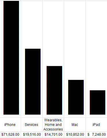
And that column, which is highlighted in yellow, is now the only one that is used in my chart. Now, the chart is cleaner and only includes the selected series rather than all three of them:

If you liked this post on Use Drop-Down Lists With Charts in Excel to Make Them Dynamic, please give this site a like on Facebook and also be sure to check out some of the many templates that we have available for download. You can also follow us on Twitter and YouTube.