Do you have multiple lists in Excel or Google Sheets that you want to combine together? With new functions such as VSTACK and HSTACK, you can do just that. In this post, I’ll show you how you can also filter out duplicates and apply sorting so that your data is organized after consolidating all of your lists.
Combining multiple stock lists into a large one
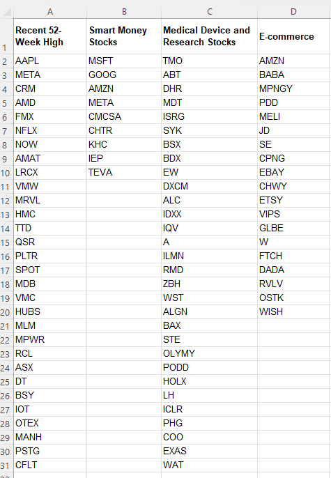
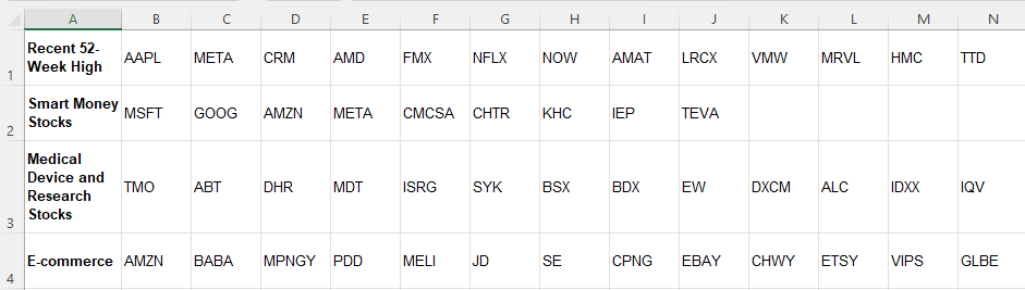
In this example, I’ll use various stock lists that I want to combine into one large list. On Yahoo Finance, you can find an assortment of different lists to help filter stocks. Below, I’ve pulled the lists of stocks that recently hit new 52-week highs, smart money stocks, medical device and research stocks, and e-commerce stocks:
The advantage of keeping the lists separate is that you can more easily update them. And by using VSTACK, you can combine these lists into a larger one so there’s no worry about having to consolidate them later on.
Based on the lists above, this is the formula that I use to combine them all together, using VSTACK:
=VSTACK(A2:A31,B2:B10,C2:C31,D2:D20)
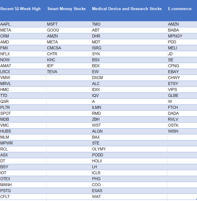
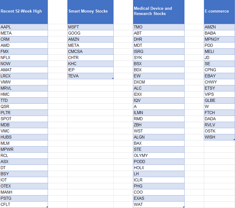
Since I don’t want to include the headers, I start from row 2. You’ll notice that I’ve hardcoded the ranges here. One way to make this more dynamic would be to use a COUNTIF or COUNTA function for the individual lists, and then use the INDIRECT function to limit the scope of the list. Another option involves converting the lists into tables. That way, you only have to list the table column and you don’t have to worry about the ranges. The one caveat here is that if you have lists that have different lengths, you’ll want to make each list its own table. Otherwise, Excel will automatically fill in the gaps with blank values:
While the data looks correct, if I were to use the VSTACK formula for these different table columns, I would get a consolidated list that involves many zero values. To keep it cleaner, it’s easier to just separate them into their own tables, and then reference them afterwards.
To reference these columns, my formula becomes much simpler:
=VSTACK(Table1[Recent 52-Week High],Table2[Smart Money Stocks],Table3[Medical Device and Research Stocks],Table4[E-commerce])
The advantage of doing it this way is that now I don’t have to worry about hardcoding the ranges, and thus, it’s easier to update.
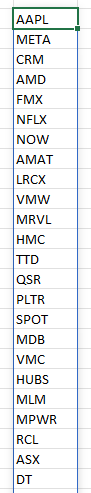
Whichever method you prefer, the end result should look like a consolidated list:
Removing duplicates and sorting the list
In some of these lists, there is some overlap. AMZN and META are two stocks that show up twice. This means that my consolidated list will include those values multiple times. To get around this, I can embed the formula within the UNIQUE function:
=UNIQUE(VSTACK(A2:A31,B2:B10,C2:C31,D2:D20))
If you also want to sort your list, then you can add the SORT function as well:
If you have the same lists but instead have them going horizontally, then you can use the HSTACK function. It works the same way as the VSTACK but as the H suggests, it will require horizontal arrays. Here are the same list of stocks as in the first example, this time transposed so that they go horizontally:
In this case, the formula for HSTACK would be as follows:
=HSTACK(B1:AE1,B2:J2,B3:AE3,B4:T4)
You can apply the same steps as for the VSTACK to eliminate duplicates and to sort the results.
These formulas work the same in Google Sheets as in Excel
Whether you’re working in Google Sheets or Excel, these formulas will be the same. The VSTACK, HSTACK, SORT, and UNIQUE functions are all available on the latest version of Excel and on Google Sheets. There is no need to change any of the formulas besides just adjusting for any difference in ranges. The formulas themselves work in the same ways, making it easy to transfer data between Google Sheets and Excel and to replicate these formulas wherever makes sense for you.
If you liked this post on How to Use VSTACK and HSTACK in Excel and Google Sheets to Consolidate Lists, please give this site a like on Facebook and also be sure to check out some of the many templates that we have available for download. You can also follow me on Twitter and YouTube. Also, please consider buying me a coffee if you find my website helpful and would like to support it.
Power Query is a powerful data transformation tool in Excel that allows you to effortlessly connect to various data sources, cleanse and manipulate data, and unlock advanced functionalities such as fuzzy matching. By leveraging the inherent “Fuzzy Lookup” feature within Power Query, you can seamlessly compare and match similar values across columns or tables using intelligent fuzzy logic algorithms. This article will highlight how you can use this functionality to help consolidate data, improve accuracy, and correct mistakes.
What is the purpose of a fuzzy lookup in Power Query?
A fuzzy lookup in Power Query refers to a powerful feature that allows you to match similar or related records within your dataset, even if they contain variations or discrepancies. Unlike an exact match that demands identical values, a fuzzy lookup takes into account the degree of similarity between values using intelligent fuzzy logic algorithms.
Imagine you have a dataset containing customer names, and you want to compare it with another dataset to identify potential matches. However, due to typos, misspellings, or differences in formatting, the exact matches may not yield the desired results. This is where a fuzzy lookup comes to the rescue.
By using a fuzzy lookup, you can overcome these obstacles. Power Query evaluates the similarity between values based on factors such as spelling variations, phonetic similarities, transpositions, and even differences in word order. This flexible approach allows you to find connections between records that might have otherwise been missed and unmatched.
There are many benefits of fuzzy lookups. They enhance data accuracy and integrity by enabling you to identify related records that might have been entered inconsistently. They can consolidate information from different sources, harmonize data formats, and facilitate a comprehensive analysis of your datasets.
Fuzzy lookups are particularly valuable when dealing with large datasets, data integration, data cleansing, or any scenario where data inconsistencies are prevalent. They provide a robust mechanism to uncover hidden associations that might have otherwise resulted in incomplete data. Leveraging the power of fuzzy lookups in Power Query can significantly improve the quality of your data analysis.
What is the difference between an exact match and a fuzzy match?
An exact match refers to a comparison between values that must be identical in every aspect, including spelling, punctuation, and formatting. It requires an exact one-to-one correspondence between the compared values.
A fuzzy lookup, however, takes a more flexible approach by considering variations, similarities, and patterns within the values being compared. It utilizes fuzzy logic algorithms to calculate the degree of similarity between the values, allowing for differences in spelling, formatting, and other factors. Here’s an example:
In this example, an exact match would fail to identify a match due to the slight difference in spelling (“Johhnson” instead of “Johnson”). However, a fuzzy lookup would recognize the similarity between the values based on the fuzzy logic algorithms, identifying them as a potential match.
While an exact match demands complete identity, a fuzzy lookup offers a more lenient approach by accommodating variations, spelling differences, abbreviations, and even phonetic similarities. It enables the discovery of relationships and connections that might otherwise be missed, allowing for more comprehensive data analysis and data integration.
The limitations of a fuzzy lookup
While fuzzy lookups in Power Query offer a powerful mechanism for matching similar records, it is important to be aware of their limitations. Understanding these limitations can help you effectively address challenges and make informed decisions when utilizing fuzzy lookups in Power Query.
Performance Impact: Performing fuzzy lookups on large datasets can have an impact on performance. Fuzzy matching involves complex algorithms that analyze the similarity between values, which requires additional computational resources. When working with extensive datasets, it is advisable to consider the potential performance implications and evaluate whether optimization techniques, such as limiting the scope of matching or using more specific matching criteria, are necessary.
Configuring Fuzzy Matching Parameters: The success of a fuzzy lookup heavily relies on properly configuring the fuzzy matching parameters. Selecting the appropriate similarity threshold and adjusting other options, such as case sensitivity or accents, is crucial. However, finding the right balance can be challenging, as overly strict or lenient parameters may result in missed matches or false positives. It often requires experimentation and fine-tuning to achieve the desired level of matching accuracy.
Data Quality and Variations: Fuzzy lookups are highly dependent on the quality and consistency of the data being matched. Inaccurate or inconsistent data, such as misspellings, abbreviations, or incomplete information, can impact the effectiveness of fuzzy matching. While fuzzy lookups can handle some degree of variation, extreme discrepancies or inconsistent patterns in the data may hinder accurate matching.
Ambiguity and Multiple Matches: In certain cases, fuzzy lookups may encounter situations where multiple records match a single value, leading to ambiguity. This can occur when there are similar records or when the matching criteria are not precise enough. Dealing with such scenarios requires additional consideration and possibly manual intervention to determine the correct matches.
Sensitivity to Dataset Size and Complexity: The effectiveness of fuzzy lookups can vary depending on the size and complexity of the dataset. Extremely large datasets or datasets with high variability in the values being matched can pose challenges. It is important to assess the scale and complexity of the data and consider alternative approaches, such as data preprocessing or dividing the task into smaller subsets, to manage the impact on performance and improve matching accuracy.
While fuzzy lookups provide valuable capabilities for identifying similar records, it is essential to be mindful of these limitations. There can be a risk of relying too heavily on fuzzy matches which results in erroneous results. By understanding and addressing these limitations appropriately, you can maximize the benefits of fuzzy lookups in Power Query and make informed decisions when incorporating them into your data analysis workflow.
Steps to do a fuzzy lookup in Power Query
Here’s a detailed overview of how to perform a fuzzy lookup in Excel:
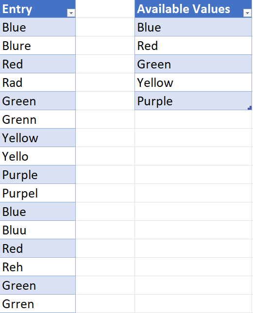
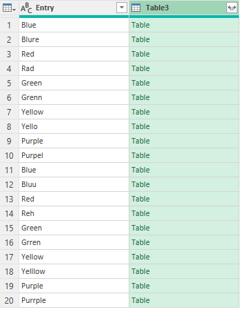
Step 1: Load your datasets into Power Query. Open Excel and go to the Data tab. Click on “Get Data” and select the appropriate option to load your datasets into Power Query. This could be from a file, a database, or any other supported data source. In this example, I have a couple of tables. One for the data entry, that contains misspellings. And another for the available values that users should have entered:
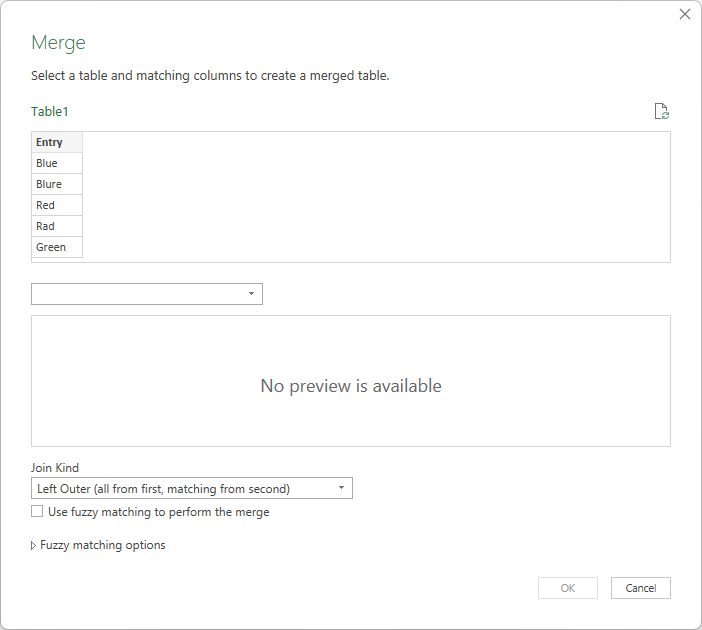
Step 2: On the data-entry table, select the Home tab and click on Merge Queries.
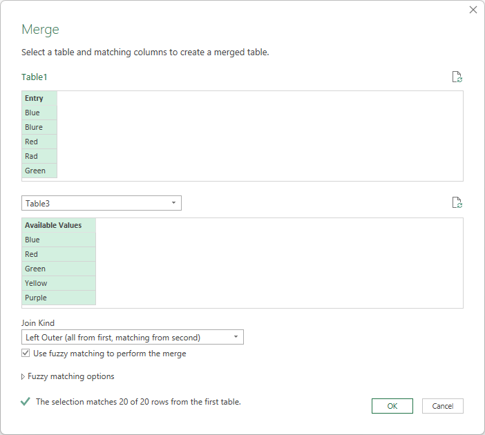
Step 3: Select the other table and highlight the fields to merge. Leave the default join as a Left Outer and below it, select the option to Use fuzzy matching to perform the merge. Upon doing this, you should see Power Query indicate that it has found more matches.
You can also open up the fuzzy matching options to select whether you want the matches to be case-sensitive, and if you want to allow it to match by combining different text parts together. You can also limit the number of matches and set the similarity threshold.
Once you’re okay with the selections, you can click on OK.
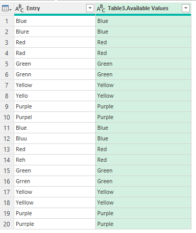
Step 4: Now, open up the and expand the table that has been merged. This will retrieve the matched values.
If everything is matched correctly, you can go ahead and click Close & Load to get the data back into Excel. If there are issues, you may want to go the previous steps to check your fuzzy matching rules, and perhaps adjust the sensitivity of the matches.
Using a Transformational Table to help fuzzy matching
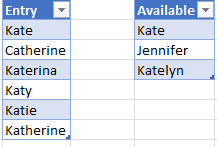
Fuzzy matches don’t always work. In some cases, you’ll need to create a transformational table to help guide Power Query. Here’s an example of when a fuzzy lookup won’t work:
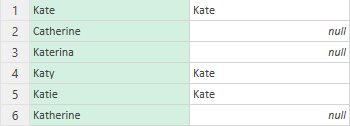
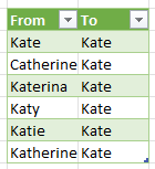
These names are similar looking and there is a big opportunity for overlap. Even when using a low sensitivity threshold, it only matches 3 of the 6 names:
The one way to definitively fix this is to create a Transformational Table for Power Query. What this does is create mapping rules. The table needs to include a ‘From’ column and a ‘To’ column such as this:
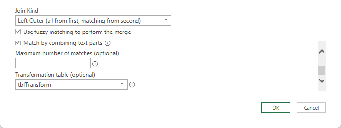
Now, when you go back to the Merge Queries dialog and adjust the Fuzzy matching options, you can specify that this is the table you want to use:
Having this table will help Power Query understand which values are related to one another. It eliminates the guesswork and can ensure everything is mapping properly. It requires a bit of extra work but it can save time in the long run. Now when using this transformational table, it matches all of the values correctly:
If you liked this post on How to Do a Fuzzy Lookup in Power Query, please give this site a like on Facebook and also be sure to check out some of the many templates that we have available for download. You can also follow me on Twitter and YouTube. Also, please consider buying me a coffee if you find my website helpful and would like to support it.
The Relative Strength Index (RSI) is a popular trading indcator that investors use for trading purposes. In this article, I’ll go over details as to what RSI is, why it’s useful, and how to calculate it in Excel.
RSI is a bounded oscillator that fluctuates between 0 and 100, providing insights to investors as to whether a stock is overbought or oversold. It compares the magnitude of recent price gains relative to recent price losses over a specified period of time, typically 14 days, and generates a value that indicates the potential for a price reversal or continuation.
The higher the losses are relative to the gains, the lower the RSI value becomes. And the opposite is also true, with the RSI value rising when a stock has been accumulating more gains than losses. Generally, an RSI value above 70 indicates an overbought condition, suggesting a potential price correction or reversal to the downside. Conversely, an RSI value below 30 indicates an oversold condition, implying a potential price bounce or reversal to the upside. Traders often use these overbought and oversold levels to identify possible entry or exit points in the market.
Why RSI Is a Useful Indicator for Traders
It’s important to note that the RSI is just one tool among many in technical analysis, and it should be used in conjunction with other indicators and analysis methods to make well-informed trading decisions. However, here are 4 reasons traders might find it useful:
1. Finding overbought and oversold levels
RSI can help investors identify buying and selling opportunities. When a stock is deeply oversold and the business is still in good shape but perhaps is down due to a bad quarter, it could be a sign to buy the beaten-down stock. In essence, it can help find market overreactions. At the same time, it can spot a stock that perhaps has become too hot when its RSI level is over 70 or 80, and that perhaps it has risen too much and too quickly.
It’s useful to also look at a stock’s historical RSI levels to gauge what kind of an opportunity it is. If it frequently dips in and out of oversold/overbought territory, it could simply be that the stock is volatile. But if it is rare for the stock to become oversold/overbought, then it could make for a good opportunity to buy or sell the stock depending on what the indicator says.
2. Measuring momentum and confirming a trend
The RSI provides insights into the strength and momentum of a price trend. When the RSI is rising and stays above 50, it indicates that buying pressure is dominant and the price trend may continue. Conversely, when the RSI is falling and stays below 50, it suggests that selling pressure is dominant and the price trend may continue downward. This information can help investors confirm the strength of a trend and make informed decisions about entering or exiting positions.
3. Identifying divergence patterns
Another valuable aspect of the RSI is its ability to identify divergence patterns. Divergence occurs when the direction of the RSI differs from the direction of the price. Bullish divergence happens when the price makes lower lows while the RSI makes higher lows, indicating a potential trend reversal to the upside. On the other hand, bearish divergence occurs when the price makes higher highs while the RSI makes lower highs, suggesting a potential trend reversal to the downside. Investors can use these divergence patterns as early warning signals of potential trend shifts and adjust their investment strategies accordingly.
4. Confirmation with other indicators
The RSI can be used in conjunction with other technical indicators to confirm signals and strengthen investment decisions. For example, if a stock shows overbought conditions based on the RSI, investors may look for additional indicators such as bearish candlestick patterns or negative volume divergences to support their decision to sell or take profits.
Other technical indicators investors can use alongside RSI
Investors often use many different indicators to make investment decisions. Here are a few commonly used indicators that can be used in conjunction with the RSI:
1. Moving Averages
Moving averages are trend-following indicators that smooth out price fluctuations over a specific period. The most commonly used moving averages are the simple moving average (SMA) and the exponential moving average (EMA). Investors often use moving averages in combination with the RSI to identify trend direction and potential support or resistance levels.
2. MACD (Moving Average Convergence Divergence)
The MACD is another trend-following momentum indicator that consists of two lines, the MACD line and the signal line. It helps identify potential buy and sell signals by measuring the relationship between two moving averages. Traders often look for convergence or divergence between the MACD and the RSI to confirm potential trend reversals or continuations.
3. Bollinger Bands
Bollinger Bands consist of a centerline (typically a moving average) and two bands that are plotted above and below it. These bands represent volatility levels. When the price reaches the upper band, it suggests that the asset is overbought, while reaching the lower band suggests oversold conditions. Combining Bollinger Bands with the RSI can provide additional insights into potential price reversals or breakouts.
4. Stochastic Oscillator
The Stochastic Oscillator is a momentum indicator that compares the closing price of an asset to its price range over a specific period. It consists of two lines, %K and %D, which oscillate between 0 and 100. Traders often look for oversold or overbought conditions on the Stochastic Oscillator in conjunction with the RSI to confirm potential trading signals.
5. Volume indicators
Volume indicators, such as On-Balance Volume (OBV) or Volume Weighted Average Price (VWAP), provide insights into the buying and selling pressure behind price movements. By analyzing volume alongside the RSI, investors can assess the strength and validity of potential price trends or reversals.
6. Fibonacci retracements
Fibonacci retracements are based on the mathematical relationships found in the Fibonacci sequence. They are used to identify potential support and resistance levels. Combining Fibonacci retracements with the RSI can help investors identify areas where a price correction or reversal may occur.
These are just a few examples of indicators that investors can use alongside the RSI. The choice of indicators depends on the investor’s trading strategy, timeframes, and personal preferences. It’s important to test and evaluate different combinations of indicators to find a system that works well for individual investment goals and risk tolerance.
Why you shouldn’t buy a stock just because the RSI is low
Buying a stock solely based on a low RSI level is not a recommended approach for several reasons:
1. It lacks context
The RSI is just one indicator and provides a snapshot of the stock’s recent price performance relative to its own historical price movements. It doesn’t take into account other fundamental factors or external market conditions that may impact the stock’s future prospects. For example, a stock may have a very low RSI because investors are selling it off due to liquidity issues or problems that may significantly impact the investing thesis behind a stock. Therefore, solely relying on the RSI without considering other relevant information may lead to an incomplete assessment of the stock’s potential.
2. False signals
The RSI is a bounded oscillator that fluctuates between 0 and 100. While an RSI below 30 may indicate an oversold condition, it doesn’t guarantee an immediate rebound or a profitable buying opportunity. Stocks can remain oversold for extended periods, and the RSI alone may not accurately predict the timing or magnitude of a price reversal. It’s essential to consider other technical and fundamental indicators to validate the potential opportunity.
3. Downtrends and value traps
A low RSI reading can sometimes be an indication of a stock in a prolonged downtrend. Just because a stock is oversold does not mean it will necessarily recover or provide substantial returns. There may be fundamental reasons behind the stock’s decline, such as poor financial performance, unfavorable industry conditions, or negative news. Investing solely based on a low RSI without understanding the underlying reasons for the low reading can lead to falling into a “value trap” not unlike how investors may buy a stock simply because its price-to-earnings multiple is low.
4. Confirmation bias
Relying solely on the RSI to make investment decisions may lead to confirmation bias, where investors seek information that supports their preconceived notions. It’s crucial to consider a broader range of indicators, conduct thorough research, and evaluate multiple factors to make well-informed investment decisions.
5. False oversold signals in strong downtrends
In strong downtrends, a stock can remain oversold for an extended period as selling pressure continues. Attempting to catch a falling knife solely based on a low RSI reading can result in further losses if the stock continues its downward trajectory. It’s important to assess the overall trend, market conditions, and other technical and fundamental factors to increase the probability of making successful investment decisions.
While the RSI can be a useful tool to identify potential opportunities, it should be considered as part of a comprehensive analysis that incorporates other indicators, fundamental analysis, and market conditions. By taking a holistic approach to investment decision-making, investors can make more well-rounded and informed choices.
How do you calculate RSI?
Here are the steps to take when determining how to calculate RSI:
1. Determine the timeframe
Traders usually use a 14-day timeframe for calculating the RSI, but it can be adjusted to suit different trading strategies and timeframes.
2. Calculate the average gain and average loss
The RSI compares the average gains and average losses over the chosen timeframe. To calculate the average gain, sum up all the positive price changes (gains) over the period and divide them by the number of periods. Similarly, calculate the average loss by summing up all the negative price changes (losses) and divide that by the number of periods.
3. Calculate the relative strength (RS)
The relative strength is the ratio of the average gain to the average loss. RS = Average Gain / Average Loss.
4. Calculate the RSI
The RSI is derived from the relative strength and is calculated using the formula: RSI = 100 – (100 / (1 + RS)).
Calculating RSI in Excel
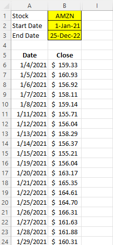
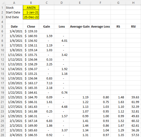
Using the STOCKHISTORY function in Excel, you can easily download a stock’s historical prices. In this example, I’ve downloaded Amazon’s stock price between the period Jan 1, 2021 and Dec 25, 2022.
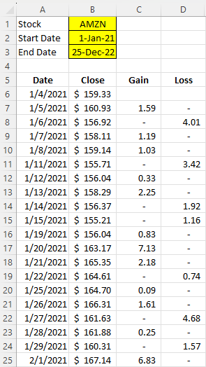
The next step is to calculate the gains and losses for each day. This just involves looking at the current closing price and the previous. If the price went down, the difference goes into the loss column. If it’s a gain, it goes into the gain column. Here’s an example of the formula for the gain column:
=IF(B7>B6,B7-B6,0)
Here’s a look at what the sheet looks like with the formulas filled in for the gain and loss columns:
Next up, I need to calculate the average gains and average losses. I’ll do this for the past 14 trading days. For the first value, I just need to calculate a simple average:
=AVERAGE(C7:C20)
For subsequent cells, however, I’ll use an exponential average. That way, I’ll apply more weighting to the the most recent calculation:
=((E20*13)+C21)/14
Next, I will calculate the RS Value. To do this, I take the average gain and divide it by the average loss:
=E20/F20
Lastly, that leaves the RSI calculation, which contains the following formula:
=100-(100/(1+G20))
With all the fields filled in, this is what the spreadsheet looks like:
If you want to follow along with the file that I’ve created, you can download it from here. You can also watch the corresponding YouTube video that goes along with this tutorial:
If you liked this post on How to Calculate the Relative Strength Index (RSI) in Excel, please give this site a like on Facebook and also be sure to check out some of the many templates that we have available for download. You can also follow me on Twitter and YouTube. Also, please consider buying me a coffee if you find my website helpful and would like to support it.
Excel has many different functions that can help you parse out text from cells. This includes the LEN, MID, LEFT, and RIGHT functions. By utilizing these and other functions, you can get just the values you want. And by determining the number of blank spaces within a cell, you can also determine the number of words that a cell contains. There are multiple ways you can count cells in Excel, I’ll start with using the easier, and newer TEXTSPLIT function.
Method 1: Counting words using the TEXTSPLIT function
The TEXTSPLIT function is available for users who have Microsoft 365 and so if you do not see that function available as you type it in, you’ll need to move to the second approach. Using the TEXTSPLIT function, you can turn a single text value in a cell into multiple cells or columns. And you can specify how you want to split a cell; which delimiter you want to use.
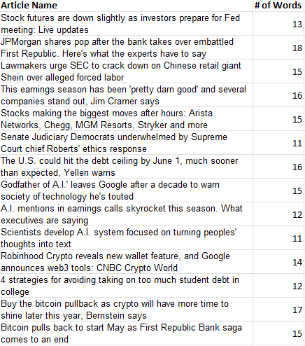
In the example of counting words, the delimiter you would use is a blank space, as specified with ” ” in the delimiter argument. Here’s a list of article titles that I am going to use for this example:
The article titles are in column A. The formula to split the text every time there is a blank space would be as follows, assuming the first value is in cell A2:
=TEXTSPLIT(A2,” “)
This formula, however, would simply put all the words in different columns. Thus, it is incomplete when your goal is to count the number of words. To fix this, the formula needs to be embedded within the COUNTA function. How COUNTA works is that it simply counts the number of nonblank values.
=COUNTA(TEXTSPLIT(A2,” “))
Copying this formula down, these are the resulting values and the number of words found in each cell:
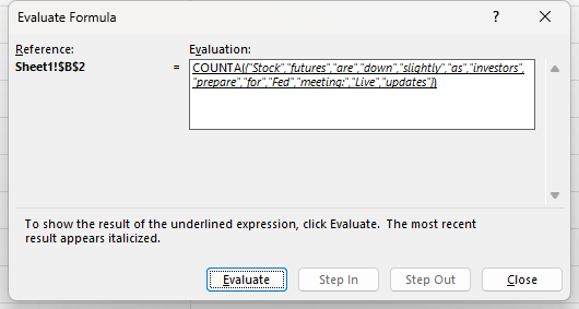
Here’s a closer look at how the formula in B2 works, using the Evaluate Formula feature in Excel:
The TEXTSPLIT function is breaking out each word as its own separate value. And the COUNTA function is then counting each one of those values. When combined, these functions allow you to count the number of words in a cell.
If you’re using Google Sheets, you can use the exact same formula as shown above, with the only difference being that instead of TEXTSPLIT, you’ll use the SPLIT function. It works in the exact same way.
Method 2: Using the LEN and SUBSTITUTE functions to count words
If you are on an older version of Excel where TEXTSPLIT isn’t available, there’s still a way that you can count the number of words within a cell. It will be a slightly more complex formula that will use the LEN and SUBSTITUTE functions.
The first part of the formula will involve counting the number of characters in a cell, which is what the LEN function does. This is accomplished through the LEN(A2) formula — assuming that A2 is where the article name is.
Next, you’ll need to use the SUBSTITUTE function to replace the blank values ” ” with an empty string that just contains two quotes: “”. To do that, the formula for that portion would be: SUBSTITUTE(A2,” “,””). This formula will need to be enclosed within a LEN function. What this accomplishes is it counts the number of characters in the cell after you’ve replaced all the blank values. If you take the total cell length and subtract this second piece, you’ll be left with the number of blank values in the text.
=LEN(A2)-LEN(SUBSTITUTE(A2,” “,””)
However, this isn’t entirely correct as you will be off by 1 word. This is because since the formula is counting the number of blanks, it won’t include the first word, which doesn’t come with a space before it. That also means if you only have one word, you’ll have a value of 0 instead of 1. To fix this, you’ll simply need to add a +1 to the end of your formula.
=LEN(A2)-LEN(SUBSTITUTE(A2,” “,””)+1
This would mean, however, that even blank cells would return a value of 1. And this would technically be the same problem when using the TEXTSPLIT function as well, since it doesn’t check for blanks, either. To correct this, you can simply add an IF function to check if the value is indeed blank. Here’s how the full formula looks:
This will return nothing if the cell is blank. If the cell isn’t blank, then it will go ahead and perform the rest of the calculation. As mentioned, this IF function can also be added to the start of the TEXTSPLIT function as well.
If you liked this post on How to Count Words in Excel, please give this site a like on Facebook and also be sure to check out some of the many templates that we have available for download. You can also follow me on Twitter and YouTube. Also, please consider buying me a coffee if you find my website helpful and would like to support it.
Net Present Value (NPV) is a financial metric used to determine the current value of a series of cash inflows and outflows. It takes into account the time value of money, which means that a dollar received in the future is worth less than a dollar received today due to factors like inflation and the opportunity cost of not having that money available to invest in other projects.
The calculation of NPV involves discounting the expected future cash flows of a project or investment back to their present value using a specified discount rate. The result is the difference between the present value of the expected cash inflows and outflows.
NPV is an important calculation because it helps you evaluate the profitability and feasibility of an investment. It can also allow you to compare the expected returns of different investment opportunities, and to make informed decisions about which projects to pursue.
If the NPV is positive, it means that the project is expected to generate more cash inflows than outflows, and thus, it’s a profitable investment opportunity. However, if the NPV is negative, the project is expected to result in a net loss and is therefore not considered a viable option.
The NPV calculation is an important tool in finance as it can help decision makers determine whether to move forward on a project.
What is the Internal Rate of Return (IRR)?
The Internal Rate of Return (IRR) is used to measure the profitability of an investment project or opportunity, often in conjunction with calculating NPV. It is the discount rate where the present value of expected cash inflows equals the present value of expected cash outflows, or when NPV is equal to 0.
IRR represents the rate of return at which an investment will break even over its lifetime. It is shown as a percentage. And if you use the IRR percentage as your discount rate in the NPV calculation, the result will be an NPV of 0.
With Excel, you can quickly calculate the IRR through a simple formula, rather than having to go through a time-consuming process that might otherwise involve trial and error.
Calculating NPV and IRR in Excel
To illustrate how to calculate NPV and IRR, I’ll use the following example. Suppose that you are investing $1,000 into a project that will generate the following cost savings:
Year 1: $50
Year 2: $100
Year 3: $250
Year 4: $300
Year 5: $600
In total, that is $1,300 in cost savings. Although that’s more than the original $1,000 investment, those savings are spread out over a period of five years. To get a true picture of whether the project is worthwhile, you need to adjust for the time value of money and adjust those amounts and calculate their present values — what their values are today. This is where the NPV function comes into play.
However, before using the NPV function, you need to determine the discount rate that you are going to use. The discount rate is important as it tells you the interest rate that you will be using when adjusting the cost savings back to today, and to calculate the present value. If the discount rate is high, then it’ll be more difficult for the NPV calculation to be positive (and hence, suggest that the investment should be taken on). And if the discount rate is too low, then it could be too easy to clear the bar and for the NPV formula to suggest the project is worthwhile.
The discount rate should be higher than the risk-free rate since you are taking on some risk, and thus, you should be compensated for doing so. If you were to use the same rate as what you could earn on a treasury bill or a bank deposit, there would be little incentive to go ahead with the project even with a positive NPV. After all, what’s the point of taking on the risk if you’re not getting a better return?
In this example, I’m using a discount rate of 5%. This is what the NPV formula will look like with all of the inputs:
=NPV(0.05,50,100,250,300,600)-1000
As you can see, the order of the values is important as that will determine how many periods each value will be discounted by. The result of this formula is a value of $71.21. It’s a positive amount, indicating that the project should be undertaken as the present value of the future cost savings offset the current investment.
To prove that calculation out, I’ll show you how this calculation could be done manually. Here, for example, is how the present value would be calculated for the $50 in cost savings that is achieved in year 1:
=50*(1+0.05)^-1
One plus the discount rate is raised to a power of negative one to bring the value back one period, using the discount rate. That returns a value of $47.619. Here are the other present value calculations:
Year 2 ($100) : $90.703
Year 3 ($250) : $215.959
Year 4 ($300) : $246.811
Year 5 ($600): $471.116
If you add all of these present values up, they total $1,071.21. And that is $71.21 more than the $1,000 initial investment, which is the same result as the NPV formula.
One thing you may be wondering is at what point does the value equal 0 — where is the breakeven? This can be calculated using the IRR formula. In Excel, this is a simple formula that just takes all the inflows and outflows. For example, if you had the negative investment amount of $1,000 in cell A1 followed by the cost savings in the the adjacent columns (until column F), then the formula for IRR would be as follows:
=IRR(A1:F1)
The end result is a value of 6.8576%. If you use this as the discount rate in the NPV calculation, you will get an NPV value of 0. This tells you that if you use a discount rate higher than this percentage, your NPV value will be negative as the level of discounting will be too high for the project to have a positive NPV value. On the other hand, anything below the IRR rate will result in a positive NPV value and thus indicate that the project should move forward.
If you liked this post on How to Calculate Net Present Value and Internal Rate of Return in Excel, please give this site a like on Facebook and also be sure to check out some of the many templates that we have available for download. You can also follow me on Twitter and YouTube. Also, please consider buying me a coffee if you find my website helpful and would like to support it.
Did you know that you can pull in emails from your Gmail account into Google Sheets? This can be useful if you don’t want to open up Gmail and do a search; you can do it right within Google Sheets. You can extract the body, subject, and other attributes. This can make it easy to scan through your messages and potentially parse out data from the body. Below, I’ll share with you the code to do this and how it works. You can also download the template if you don’t want to create it yourself.
Creating the sheet and setting up the variables
You probably don’t want to pull every email into your Google Sheets file. For that reason, it’s important to set up variables that will allow you to do a search. In my template, I’ve got an area to search by the subject and by label, with the named ranges being keysubject, and keylabel, respectively. This is where the search terms go. And this is similar to how you would search within Gmail, searching by both the subject and the label.
The Google Apps Script code
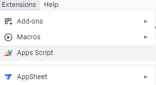
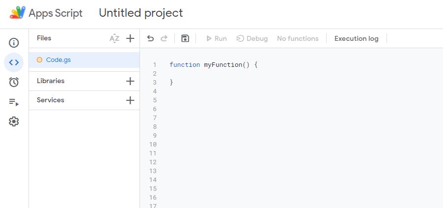
To attach the code to your Google Sheets file, you’ll need to go the Extension tab and select the option for Apps Script
From there, you should see a new tab open that gives you an untitled project where you can enter in code:
The function name can remain as default, the key is to copy the code within the curly brackets, { and }. The code that I use for the function to pull in emails is as follows:
var ss = SpreadsheetApp;

var sht = ss.getActiveSheet();

var lastrow = sht.getLastRow();

var k = 6;

var rng = sht.getRange(k,1,lastrow,4);

rng.clearContent();

var emailstring = 'https://mail.google.com/mail/u/0/#inbox/';

var emaillink;

var keysubject = "subject:(" + sht.getRange("keysubject").getValue().toString()+")";

var keylabel = sht.getRange("keylabel").getValue().toString();

var searchquery = GmailApp.search(keylabel + " " + keysubject);

var allthreads = GmailApp.getMessagesForThreads(searchquery);

var emaildate;

var emailsubject;

for (var i=0; i<allthreads.length; i++) {

  var activethread = allthreads[i];

  for (var j=0; j<activethread.length; j++) {

            emaildate = activethread[j].getDate();

            emailsubject = activethread[j].getSubject();

            emailbody = activethread[j].getPlainBody().substring(0,300);

            emailID = activethread[j].getId();

            sht.getRange(k,1).setValue(emaildate);

            sht.getRange(k,2).setValue(emailsubject);

            emaillink = emailstring + emailID

            sht.getRange(k,3).setValue(emaillink);

            sht.getRange(k,4).setValue(emailbody);

          k +=1

  }

}
There are a couple things to note in the code, should you want to change the layout of your file and where you want the data to go.
At the beginning of the code, there is a variable, k. It determines the starting row for the data. In my code, the value is set to 6 because my headers are in row 5. That means row 6 is the starting point for the data. If you want your headers to be in row 10, for example, you’ll want to set the k value to 11, so that it starts on the following row.
Towards the end of the code, you’ll see where the values are being populated. For example, the date of the email is being populated with the following line:
sht.getRange(k,1).setValue(emaildate);
The k variable is specified at the beginning of the code. However, you can change the the column number (1) at this line. Do not change the k value here. If you do, then your data will be overwritten in the same row over and over. This is because in this part of the code the function is doing a loop and it will increment the k value. And so if you want to change it, you need to do it when the k variable is first set up — before the loop.
If, however, you want to change the column that the value is going to, this is the correct place to do so. For example, suppose you don’t want the date going into column A, then you can change the column number. For example, if you want to change it to column B, then you would change (k,1) to (k,2).
If there are certain fields that you don’t want to be populating, then you can also just remove those lines entirely.
For the body of the email, you may want to adjust how much of it gets pulled into the file. Too much text can force your column to get spread out. And if there are line breaks, the row can also get expanded. In my code, I’ve set the limit to the first 300 characters. However, you can change that by adjusting the following line of code:
One last note before moving on from this section — remember to save any changes before trying to run the macro again. If you don’t save, then the changes won’t be applied when you run the macro.
Adding a button to trigger the macro
The one thing that you may want to do after adding the code is to create a button on your spreadsheet to trigger it. Otherwise, you’ll need to go to the Apps Script tab and click the run button each time, which isn’t practical.
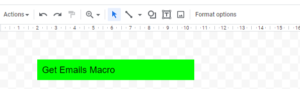
Instead of doing that, select the Insert button on the Google Sheets file and select Drawing. You’ll have a blank canvas where you can create a button. Here, you can select an option to create a shape and enter text within it. You can apply different colors to also make it stand out. One you’re done designing it, click on Save and close and the button will be on your spreadsheet.
Once it’s within your spreadsheet, you’ll see that there will be three dots off to the right of the button. This is where you can assign your button to the macro that you’ve created. In my example, my function is called getEmails and that’s what I’ll enter when I’m assigning the button to a script;
If you’ve used a different function name, you will need to enter it above, and then click OK. Don’t enter the parentheses, (), which come after the function in Apps Script. Once you’ve assigned the script to the button, you can now click on the button and run the function.
This will only run on the email account you’re logged in on
If you’re like me and you have multiple Gmail accounts, the one thing you need to know is that this will macro will run on the account you’re logged in on; it won’t be able to toggle between different accounts for you.
If you liked this post on How to Get Emails Into Google Sheets, please give this site a like on Facebook and also be sure to check out some of the many templates that we have available for download. You can also follow me on Twitter and YouTube. Also, please consider buying me a coffee if you find my website helpful and would like to support it.
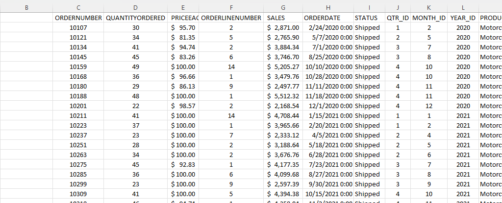
If you’re an accountant, you know that working with large amounts of data can be a daunting task. But with Excel, that work can get a whole lot easier and more efficient. Understanding Excel’s advanced features and functions can improve productivity, reduce errors, make your work more accurate, and most importantly — save you time. Below, I’ll go over some of the most important Excel functions that accountants should know, and provide examples of how to use them. For this example, I’ll use the following spreadsheet. Feel free to download it and follow along with the calculations.
1. SUM
The SUM function is a basic but essential function in Excel. It allows you to add up a range of values, which is helpful when calculating totals, such as revenue, expenses, and profits. Suppose you have a spreadsheet with sales data. In the above example, the total sales are in column G. If you wanted to sum up the entire column, the formula would be as follows: =SUM(G:G)
2. AVERAGE
The AVERAGE function calculates the average of a range of values. It is useful when analyzing data and preparing financial statements. In the above example, suppose you wanted to calculate what the average sale was. To do this, you can just use the AVERAGE function on column G, similar to the SUM function before. Here’s the formula: =AVERAGE(G:G)
3. IF
The IF function allows you to test a condition and return one value if the condition is true and another value if the condition is false. This can be useful because it can send your formulas to the next level. By knowing to use the IF function, you could also use SUMIF, AVERAGEIF, and many other functions that involve an if statement. In the above example, let’s say you only wanted to know if a value in cell M2 was part of the Motorcycles product line. The formula would be as follows: =IF(M2=”Motorcycles”,1,2). If it is part of Motorcycles, you would have a value of 1, otherwise, it would be 2.
4. SUMIF
By knowing the SUM and IF functions, you can combine them together with SUMIF, which is an incredibly popular function. It gives you a quick way to tally up the totals that meet a criteria. For example, let’s say you want all sales that relate to the Motorcycles category. The formula for that would be as follows: =SUMIF(M:M,”Motorcycles”,G:G). If the criteria is met in column M, then the formula will sum up the corresponding values in column G. There’s also the super-powered SUMIFS function, which allows you to combine multiple criteria.
5. EOMONTH
The EOMONTH function calculates the last day of the month for a specified number of months in the future or past. It is useful when working with data that is organized by date. For accountants, this can be useful when you’re calculating when something is due. Let’s say in this example, we need to calculate the date orders need to go out on, and that needs to be the end of the next month. Using the ORDERDATE field in column H, here’s how that calculation would look in the first cell, which would then be copied down for the rest: =EOMONTH(H2,1)
6. TODAY
The TODAY function is helpful for accountants in calculating deadlines and knowing how many days are remaining or past a certain date. Suppose that you wanted to know how many days have past since the ORDER DUE DATE that was calculated in the previous example. Rather than entering in a static date that every day you would need to change, you can just use the TODAY function. Here’s how a formula calculating the days since the deadline for the first cell would look like, assuming the due date is in column N: =TODAY()-N2. The next day you open up the workbook, the calculations will update to reflect the current date; there’s no need to make any changes. There are many more date calculations you can do in Excel.
7. FV
The FV function calculates the future value of an investment based on a fixed interest rate and a regular payment schedule. You can use it to calculate the future value of an investment or savings account. Let’s say that you wanted to save $10,000 per year and expect to earn a return of 5% per year on that investment. Using the FV calculation, you can do that with the following formula: =FV(0.05,5,-10000). If you don’t enter a negative for the payment amount, the formula will result in a negative value. You can also specify whether payments happen at the beginning of a period (1) or end (0 — this is the default) with the last argument in the function.
8. PV
The PV function lets you do the opposite and work backwards from a future value to the present. Knowing that the calculation in example 7 returns a value of $55,256.31, that can be used in the PV calculation to check our work: =PV(0.05,5,10000,-55256.31). The formula returns a value of 0, which is correct, as there was no starting value in the FV calculation.
9. PMT
The PMT function calculates the periodic payment required to pay off a loan with a fixed interest rate over a specified period. It is helpful when determining the monthly payments required to pay off a loan or mortgage. Let’s take the example of a mortgage payment where you need to pay down $500,000 over the period of 30 years, in monthly payments. At a 5% interest rate, here’s what the payment calculation would be: =PMT(0.05/12,12*30,-500000,0). Here again the ending value needs to be a negative to avoid a negative value in the result. And since the payments are monthly, the periods need to be multiplied by 12 and the interest rate is dividend by 12.
10. VLOOKUP
The VLOOKUP function allows you to search for a value in a table and return a corresponding value from another column in the same row. It’s one of the most common Excel functions because of how useful and easy to use it is. It is helpful when working with large data sets and performing data analysis. Let’s suppose in this example that you want to find the sales related to order number 10318. The formula for that calculation might look like this: =VLOOKUP(10318,C:G,5,FALSE). In a VLOOKUP function, you need to specify the column number you want to extract from, which is what the 5 represents. If you’re using Office 365, you can also use the newer, flashier XLOOKUP function. I put VLOOKUP on this list because it’ll work on older versions of Excel — XLOOKUP won’t.
11. INDEX
The INDEX function allows you to return a value from a data set by specifying the row and column number. It’s also helpful if you just want to return data from a single row or column. For example, the sales column is in column G. If I know the order number is on row 20 (which relates to order number 10318), this formula would do the same job as the VLOOKUP in the previous example: =INDEX(G:G,20,1).
12. MATCH
The MATCH function allows you to find the position of a value within a range of cells. Oftentimes, Excel users deploy a combination of INDEX and MATCH instead of VLOOKUP due to its limitation (e.g. VLOOKUP can’t extract values to the left of the lookup field). In the previous example, you had to specify the row belonging to the order number. But if you didn’t know it, you could use the MATCH function within the INDEX function. The MATCH function would look like this: =MATCH(10318,C:C,0). Placed within an INDEX function, it can replace the argument where in the previous example, we set a value of 20: =INDEX(G:G,MATCH(10318,C:C,0),1). By doing this, you have a more flexible version of the VLOOKUP function. You can also create dynamic formulas using INDEX and MATCH that use lookups for both the column and row.
13. COUNTIF
The COUNTIF function allows you to count the number of cells in a range that meet a specified condition. Let’s count the number of values in the data set that are Motorcycles. To do this, you would enter the following formula: =COUNTIF(M:M,”Motorcycles”).
14. COUNTA
The COUNTA function is similar to the previous function, except it only counts the number of non-empty cells. With no criteria, it is helpful to just the total number of values within a range. To calculate how many cells are in this data set, you can use the following formula: =COUNTA(C:C). If there are no gaps in data, then the result should be the same regardless of which column is used. And when combined with the UNIQUE function, you can have an easy way to count the number of unique values.
15. UNIQUE
The UNIQUE function returns a list of unique values within a range, and it’s a much easier method than the old-school way of extracting unique values. If you wanted to extract all the unique product lines in column M, you would enter the following formula: =UNIQUE(M:M). If, however, you just wanted to count the number of unique values, you could embed it within the COUNTA function as follows: =COUNTA(UNIQUE(M:M)). You can adjust your range if you don’t want to include the header.
This is just a sample of some of the useful Excel functions that accountants can utilize. If you are familiar with them, you’ll put yourself in a great position to improve the efficiency of your workflow and make your spreadsheets easier to use. Plus, you can confidently say that you are highly competent with Excel, which can make your resume more attractive and make you better suited for accounting jobs that require advanced Excel skills — and there are many of them that do!.
If you liked this post on 15 Excel Functions Accountants Should Know, please give this site a like on Facebook and also be sure to check out some of the many templates that we have available for download. You can also follow me on Twitter and YouTube. Also, please consider buying me a coffee if you find my website helpful and would like to support it.
If you’ve ever downloaded data and received dates in the wrong format, it can be a challenge to fix. If your regional settings are month/day/year but in a spreadsheet they are in day/month/year format, then odds are they will be reading in a text format rather than date. The one exception is when you’re dealing with month and day values that are 12 or less, and thus, they could be both month or day values. In those cases, the values are still reading as dates, but they are still incorrect. Here’s how you can fix all of these issues by using a formula.
Converting text date formats using TEXTSPLIT and INDEX
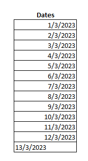
Suppose you have the following values, which are for March 2023:
These dates are not in the month/day/year format. However, only the value that has a 13 at the start is aligned to the left — indicating that it’s a text value. The others are recognized as dates, even though they are in the wrong format. This is what can make this calculation tricky, to accommodate both situations — but it’s not impossible.
First, let’s deal with the values that are in text. For these ones, their values just need to be parsed out. In the past, you could do this with a complicated series of LEN, MID, LEFT, and RIGHT functions. However, thanks to the relatively new TEXSPLIT function, it’s easier to do that.
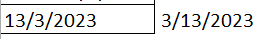
Here’s how you would parse out the data if it’s in a text format, such as in the last instance (March 13), which is in cell A14:
=TEXTSPLIT(A14,”/”)
This formula will break out the data into an array:
This isn’t the final solution, as this would still require another formula to pull these values into a date. And to accomplish that, this is where the INDEX function comes into play. Since there are three values here, using INDEX, you can select which value goes in which argument for the DATE function.
For instance, the following formula would extract the first value before the /, which is the number 13:
=INDEX(TEXTSPLIT(A14,”/”),1,1)
For the second number, 3, the column argument needs to change to a 2, to get the second column in the array:
=INDEX(TEXTSPLIT(A14,”/”),1,2)
And for the last one, the column would be set to 3:
=INDEX(TEXTSPLIT(A14,”/”),1,3)
Together, these values can be put within a DATE function. The arguments in the DATE format are in the following order: year, month, day. That means that last value in the array (position 3) needs to be first, followed by the second position (the month), and the last position (for the day). Here’s how that formula looks:
It’s the same formula repeated but referencing different column positions. And now, the formula gives me the date in the correct month/day/year format:
However, this formula won’t work on the other values; they will result in errors since those are date values and only display slashes but don’t actually contain them the way a text value does. However, the solution for these formulas is even easier.
How to rearrange date values
Since the below cells read as date values, we can reference their respective month, day, and year values, and simply put them back into the DATE function.
The first value is the day value, followed by the month, and then the year. However, my regional settings are set to month/day/year format. That means if these cells are reading as date values, which they are, then that means the first value is going to be the month. By using the MONTH function, I can get that first value. But the key is, when I’m creating a new formula and using the DATE function, I will need to put that value in the argument that relates to the day. This can be a bit tricky and remember, if your regional settings are different from mine, you will need to alter your formula to ensure the right value is going into the right argument.
Similarly, for the second value (which corresponds to the day in my regional settings), I will use the DAY function to get that value. But I will actually put it in the month argument.
Lastly, the YEAR function will extract the year and go into the same year argument position, since month/day/year and day/month/year have the same position for the year. Here’s how this formula looks in its entirety, grabbing all the different values:
=DATE(YEAR(A2),DAY(A2),MONTH(A2))
By copying the formulas, the date formats now look correct:
Combining the formulas
There’s just one left piece left in all of this, and that’s combining the two formulas so they can accommodate both situations: when the data is in text format, and when it’s reading as a date. This can be done by using the ISTEXT function, to check if a value is reading as text or not. If it’s a text value, then it will use the TEXTSPLIT function. Otherwise, it will simply reposition the date values. Here’s the formula that will factor in both situations:
Now, this one formula can be used on all of the cells, whether they are in date or text format.
If you liked this post on How to Convert Date Formats in Excel, please give this site a like on Facebook and also be sure to check out some of the many templates that we have available for download. You can also follow me on Twitter and YouTube. Also, please consider buying me a coffee if you find my website helpful and would like to support it.
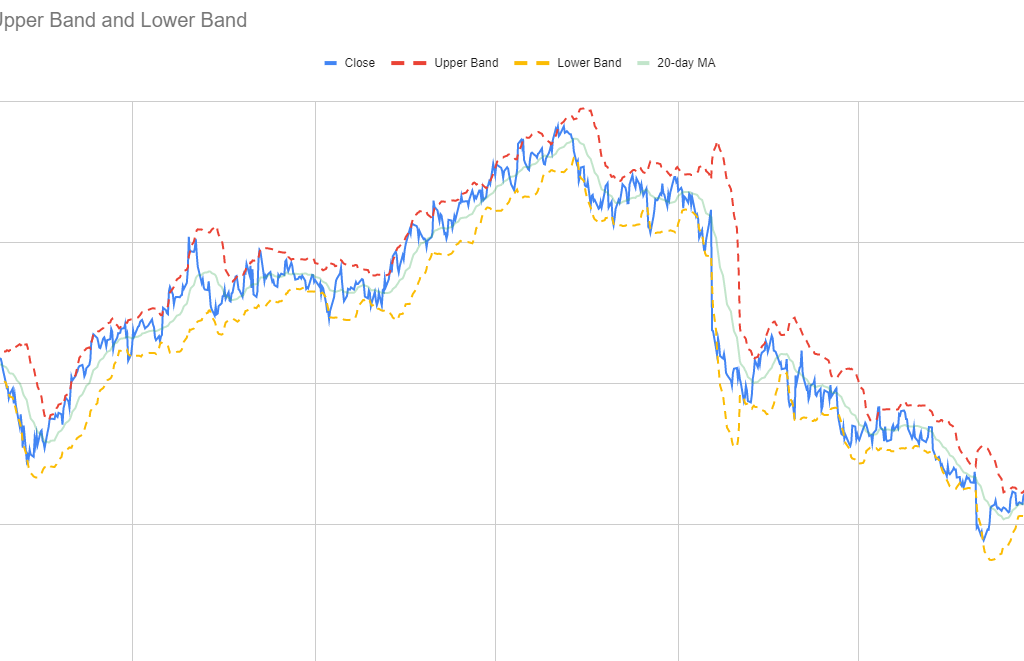
Bollinger Bands are used in technical analysis to help calculate and measure volatility. There are three bands that are included in chart: a moving average, and a lower and upper band. Normally, the upper and lower band are set to be within two standard deviations of the moving average. The standard deviation helps measure volatility and determines the width of the bands. As volatility increases, the band widens, and the opposite happens when volatility decreases.
The Bollinger Bands are often used by traders to identify opportunities for when to buy or sell a stock. If a stock price gets closer to the upper band, then it is considered to be overbought, and hence, this can be a time to sell. If, on the other hand, it is approaching the lower band, then it is oversold, and it may be an opportune time to buy. A similar tool that traders may also use is the Relative Strength Index, as that too tracks momentum and helps traders identify when a stock is overbought and oversold.
Why should you use Bollinger Bands?
Traders may use Bollinger Bands for a variety of reasons:
To identify buying and selling opportunities, such as when a stock is overbought or oversold. However, it’s important not to be overly reliant on a single indicator and it’s a good idea to also review other tools in conducting technical analysis to help confirm your trading decision.
Bollinger Bands can help gauge volatility. When the volatility is high, there is an opportunity for traders to take advantage of a large spread. With a large spread, there are more opportunities to buy low and sell high than there are when volatility is low and price is trading within just a narrow range.
Traders may also use Bollinger Bands to spot trends in the market as the bands will slope in a similar direction to price. This can help potentially identify buying and selling opportunities based on the stock’s trajectory.
How to create and chart Bollinger Bands
The process for creating a chart to show Bollinger Bands in Excel and Google Sheets is similar — the main difference is in how to pull in the stock price. The steps below go over the steps specific to Google Sheets:
Start with downloading the stock prices. In my example, I have downloaded the stock price for Meta Platforms going back to 2020. This was done using the GOOGLEFINANCE function in Google Sheets, and the formula is as follows: =GOOGLEFINANCE(“meta”,”price”,”1/1/2020″,today())
Calculate the 20-day moving average from the closing prices. This is done using the AVERAGE function. Assuming the closing prices start from cell B4, the formula would be as follows: =AVERAGE(B4:B23). Copy the formula down to all the cells.
Calculate the standard deviation using the STDEV function. This is also based on the last 20 closing prices and is copied down to the bottom of the data set. This is the formula to calculate the standard deviation based on this example: =STDEV(B4:B23).
Calculate the Upper Band. Do this by multiplying the standard deviation by 2, and adding that to the 20-day moving average. Assuming the 20-day moving average is in cell C23 and the standard deviation is in cell D23, this is what the formula would look like: =C23+D23*2
Calculate the Lower Band. For this, multiply the standard deviation by -2, and add that to the 20-day moving average. Based on the above assumptions, the formula would be as follows: =C23+D23*-2
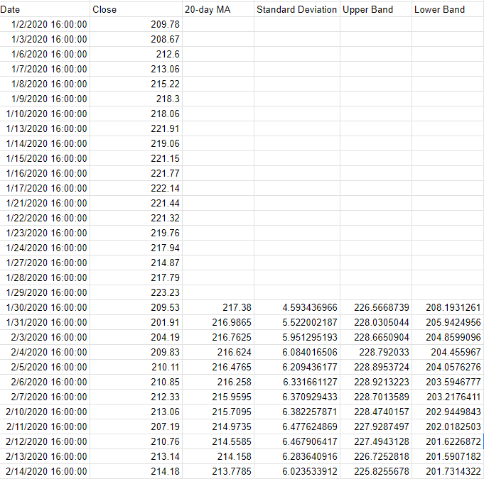
Once all those formulas are entered, your data set should look something like this:
Next, create a line chart to show the values on a graph. Then apply any formatting (e.g. dotted lines, colors, etc) and you should have a visual that looks like this:
If you liked this post on How to Create and Chart Bollinger Bands in Google Sheets and Excel, please give this site a like on Facebook and also be sure to check out some of the many templates that we have available for download. You can also follow us on Twitter and YouTube.
Want to show your data in reverse order, and want to do so without having to sort it? Using just a formula, you can change the way your data looks. Instead of going from oldest to newest, you can display it from newest to oldest. And you don’t have to alter your existing data set to do it. In this post, I’ll show you can how can flip your data through just a single formula.
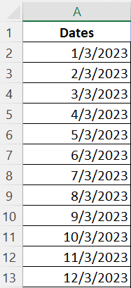
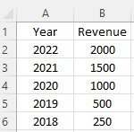
In the below example, I have data going in descending order by year.
If I wanted to change the order so that it’s in ascending order, I could use the sort button. But what if you needed to keep the data the way it is and I just wanted to put in different order, say for the sake of a chart or report. I can accomplish this using the functions INDEX, ROW, and COUNTA. Here’s how it works.
Creating the formula to flip data
The first function I’m going to use is the INDEX function. This is important because this function will include all the data that I need. Since my data is in the range A1:B6, I’ll start with a formula to get the years in column A and reverse them. The formula will start as follows
=INDEX(A$1:A$6
I’m freezing the row numbers because I want to ultimately copy this formula over to the revenue column, and flip those values as well. In the next part of my formula, I will need to grab a count of the values in my range. This can be achieved by using the COUNTA function:
=INDEX(A$1:A$6,COUNTA(A$1:A$6)
The above formula would grab the last value in the range. And while that’s technically what I want, the formula wouldn’t work if I were to copy it down. Thus, I need to add a 1 to it and I also need a way to also deduct 1 — for the first instance, anyway. To make it dynamic, I’m going to use the ROW function.
=INDEX(A$1:A$6,COUNTA(A$1:A$6)+1-ROW(A1))
How this works is that the formula will grab a count of the rows in the data set. Then the formula will add 1 but it will also deduct 1 using the ROW function. In this first formula, my value will be 6 — the same as the count of cells. However, if I drag it down, the formula for the next cell will be as follows:
=INDEX(A$1:A$6,COUNTA(A$1:A$6)+1-ROW(A2))
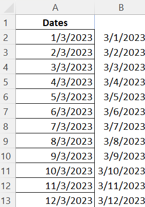
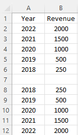
In the above formula, I’ll now be deducting 2 since the row value of A2 is 2. In this case, the row value I will be extracting is 5. The COUNTA function returns value of 6, then 1 is added, and the ROW function deducts 2. By dragging this formula down, it will now continue going backwards and so that the last value will be the first row. If I also copy this over to column B for revenue, I will now have both columns flipped and going in the opposite direction:
If you liked this post on How to Flip Your Data in Excel Without Sorting, please give this site a like on Facebook and also be sure to check out some of the many templates that we have available for download. You can also follow us on Twitter and YouTube.